Sample space and probability
library(tidyverse)
library(broom)
library(patchwork)

options(digits = 3)
set.seed(1234)
theme_set(theme_minimal())
Model of probability
- Sample space - set of all things that could happen
- Events - subsets of the sample space
- Probability - chance of an event
Sample space
The sample space as the set of all things that can occur. We will collect all distinct outcomes into the set \(\Omega\). Examples include:
- House of Representatives - elections every 2 years
- One incumbent: \(\Omega = \{W, N\}\)
- Two incumbents: \(\Omega = \{(W,W), (W,N), (N,W), (N,N)\}\)
- 435 incumbents: \(\Omega = 2^{435}\) possible outcomes (permutations)
- Number of countries signing treaties
- \(\Omega = \{0, 1, 2, \ldots, 194\}\)
- Duration of cabinets
- All non-negative real numbers: \([0, \infty)\)
- \(\Omega = \{x : 0 \leq x < \infty\}\)
- All possible \(x\) such that \(x\) is between 0 and infinity
The sample space must define all possible realizations.
Events
Events are a subset of the sample space:
\[E \subset \Omega\]
- Plain English: outcomes from the sample space, collected in a set
- Congressional election example
- One incumbent
- \(E = W\)
- \(F = N\)
- Two incumbents
- \(E = \{(W, N), (W, W) \}\)
- \(F = \{(N, N)\}\)
- 435 incumbents
- Outcome of 2016 election - one event
- All outcomes where Dems retake control of the House - one event
- One incumbent
- Notation: \(x\) is an element of a set \(E\) \[x \in E\] \[\{N, N\} \in E\]
Event operations
\(E\) is a set, or a collection of distinct objects. We can perform operations on sets to create new sets. Consider two example sets:
- \(E = \{ (W,W), (W,N) \}\)
- \(F = \{ (N, N), (W,N) \}\)
\(\Omega = \{(W,W), (W,N), (N,W), (N,N) \}\)
Operations determine what lies in the new set \(E^{\text{new}}\).
- Union: \(\cup\)
- All objects that appear in either set (OR)
- \(E^{\text{new}} = E \cup F = \{(W,W), (W,N), (N,N) \}\)
- Intersection: \(\cap\)
- All objects that appear in both sets (AND)
- \(E^{\text{new}} = E \cap F = \{(W,N)\}\)
- Complement of set \(E\): \(E^{c}\)
- All objects in \(S\) that are not in \(E\)
- \(E^{c} = \{(N, W) , (N, N) \}\)
- \(F^{c} = \{(N, W) , (W, W) \}\)
- What is \(\Omega^{c}\)? - an empty set \(\emptyset\)
- Suppose \(E = {W}\), \(F = {N}\). Then \(E \cap F = \emptyset\) (there is nothing that lies in both sets)
Probability
- Probability is the chance of an event occurring
- \(P\) is a function
- The domain contains all events \(E\)
Three axioms
All probability functions \(P\) satisfy three axioms:
- Nonnegativity: For all events \(E\), \(0 \leq P(E) \leq 1\)
- Normalization: \(P(S) = 1\)
- Additivity: For all sequences of mutually exclusive events \(E_{1}, E_{2}, \ldots,E_{N}\) (where \(N\) can go to infinity): \[P\left(\cup_{i=1}^{N} E_{i} \right) = \sum_{i=1}^{N} P(E_{i} )\]
- Any countable sequence of mutually exclusive events can be added together to generate the probability of any of the mutually exclusive events occurring
Basic examples
Rolling the dice
Consider the experiment of rolling a pair of 4-sided dice. We assume the dice are fair, and we interpret this assumption to mean that each of the sixteen possible outcomes [pairs \((i,j)\) with \(i,j = 1,2,3,4\)] has the same probability of \(1/16\). To calculate the probablity of an event, we must count the number of elements of the event and divide by 16 (the total number of possible outcomes). Here are some event probabilities calculated this way:
\[ \begin{aligned} \Omega &= \{(1,1), (1,2), (1,3), (1,4), (2,1), (2,2), (2,3), (2,4), \\ &\quad (3,1), (3,2), (3,3), (3,4), (4,1), (4,2), (4,3), (4,4) \} \end{aligned} \]
\[ \begin{aligned} \Pr (\text{the sum of the rolls is even}) &= 8/16 = 1/2 \\ \Pr (\text{the sum of the rolls is odd}) &= 8/16 = 1/2 \\ \Pr (\text{the first roll is equal to the second}) &= 4/16 = 1/4 \\ \Pr (\text{the first roll is larger than the second}) &= 6/16 = 3/8 \\ \Pr (\text{at least one roll is equal to 4}) &= 7/16 \end{aligned} \]
Romeo and Juliet
Romeo and Juliet have a date at a given time, and each will arrive at the meeting place with a delay between 0 and 1 hour, with all pairs of delays being equally likely. The first to arrive will wait for 15 minutes and will leave if the other has not yet arrived. What is the probability that they will meet?
Click for the solution
Let us use as the sample space the unit square, whose elements are the possible pairs of delays for the two of them. Our interpretation of “equally likely” pairs of delays is to let the probability of a subset of \(\Omega\) be equal to its area. This probability law satisfies the three probability axioms. The event that Romeo and Juliet will meet is the shaded region in the figure below, and its probability is calculated to be \(7/16\).
data_frame(x = seq(from = 0, to = 1, by = 0.001),
           ylow = -.25 + x,
           yhigh = .25 + x) %>%
  ggplot(aes(x = x)) +
  geom_line(aes(y = ylow)) +
  geom_line(aes(y = yhigh)) +
  geom_ribbon(aes(ymin = ylow, ymax = yhigh), alpha = .2) +
  annotate(geom = "text", x = .5, y = .5, label = "M") +
  scale_x_continuous(breaks = c(0, .25, 1)) +
  scale_y_continuous(breaks = c(0, .25, 1)) +
  coord_fixed(xlim = c(0, 1),
              ylim = c(0, 1),
              expand = FALSE) +
  labs(x = "Romeo",
       y = "Juliet") +
  theme_classic() +
  theme(panel.border = element_rect(color = "black", fill = NA, size = 1))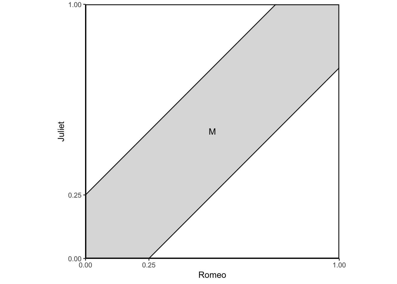
The event that Romeo and Juliet will arrive within 15 minutes of each other is
\[M = \{ (x,y) \mid | x - y | \leq 1/4, 0 \leq x \leq 1, 0 \leq y \leq 1 \}\].
The area of \(M\) is 1 minus the area of the two unshaded triangles, or \(1 - (3/4) \times (3/4) = 7/16\). Thus the probability of meeting is \(7/16\).
Conditional probability
Social scientists almost always examine conditional relationships
- Given opposite Party ID, probability of date
- Given low-interest rates probability of high inflation
- Given “economic anxiety” probability of voting for Trump
Intuition:
- Some event has occurred: an outcome was realized
- And with the knowledge that this outcome has already happened
- What is the probability that something in another set happens?
Definition:
Suppose we have two events, \(E\) and \(F\), and that \(P(F)>0\). Then,
\[ \begin{eqnarray} P(E|F) & = & \frac{P(E\cap F ) } {P(F) } \end{eqnarray} \]
- \(P(E \cap F)\): Both \(E\) and \(F\) must occur
- \(P(F)\) normalize: we know \(P(F)\) already occurred
Examples
Elections
- Example 1
- \(F = \{\text{All Democrats Win} \}\)
- \(E = \{\text{Nancy Pelosi Wins (D-CA)} \}\)
- If \(F\) occurs then \(E\) most occur, \(P(E|F) = 1\)
- Example 2
- \(F = \{\text{All Democrats Win} \}\)
- \(E = \{ \text{Louie Gohmert Wins (R-TX) }\)
- \(F \cap E = \emptyset \Rightarrow P(E|F) = \frac{P(F \cap E) }{P(F)} = \frac{P(\emptyset)}{P(F)} = 0\)
- Example 3: incumbency advantage
- \(I = \{ \text{Candidate is an incumbent} \}\)
- \(D = \{ \text{Candidate Defeated} \}\)
- \(P(D|I) = \frac{P(D \cap I)}{P(I) }\)
- In words – the probability that a candidate is defeated given that the candidate is an incumbent is equal to the probability of being defeated AND being an incumbent divided by the probability of being an incumbent
Design teams
A conservative design team, call it \(C\), and an innovative design team, call it \(N\), are asked to separately design a new product within a month. From past experience we know:
- The probability that team \(C\) is successful is \(2/3\).
- The probability that team \(N\) is successful is \(1/2\).
- The probability that at least one team is successful is \(3/4\).
Assuming that exactly one successful design is produced, what is the probability that it was designed by team \(N\)?
Click for the solution
There are four possible outcomes here, corresponding to the four combinations of success and failure of the two teams:
- \(SS\): both succeed
- \(SF\): \(C\) succeeds, \(N\) fails
- \(FS\): \(C\) fails, \(N\) succeeds
- \(FF\): both fail
We were given that the probabilities of these outcomes satisfy:
\[\Pr (SS) + \Pr (SF) = \frac{2}{3}, \quad \Pr (SS) + \Pr (FS) = \frac{1}{2}, \quad \Pr (SS) + \Pr (SF) + \Pr (FS) = \frac{3}{4}\]
From these relations, together with the normalization equation:
\[\Pr (SS) + \Pr (SF) + \Pr (FS) + \Pr (FF) = 1\]
we can obtain the probabilities of individual outcomes:
\[ \begin{aligned} \Pr (FF) &= 1 - [\Pr (SS) + \Pr (SF) + \Pr (FS)] = 1 - \frac{3}{4} &= \frac{1}{4} \\ \Pr (SF) &= \frac{3}{4} - [\Pr (SS) + \Pr (FS)] = \frac{3}{4} - \frac{1}{2} &= \frac{1}{4} \\ \Pr (FS) &= 1 - [\Pr (SS) + \Pr (SF)] - \Pr (FF) = 1 - \frac{2}{3} - \frac{1}{4} &= \frac{1}{12} \\ \Pr (SS) &= 1 - \Pr (SF) - \Pr (FS) - \Pr (FF) = 1 - \frac{1}{4} - \frac{1}{4} - \frac{1}{12} &= \frac{5}{12} \end{aligned} \]
The desired conditional probability is:
\[ \Pr (FS | \{ SF, FS \}) = \frac{\frac{1}{12}}{\frac{1}{4} + \frac{1}{12}} = \frac{\frac{1}{12}}{\frac{3}{12} + \frac{1}{12}} = \frac{\frac{1}{12}}{\frac{4}{12}} = \frac{12}{12 \times 4} = \frac{1}{4} \]
Difference between \(P(A|B)\) and \(P(B|A)\)
\[ \begin{eqnarray} P(A|B) & = & \frac{P(A\cap B)}{P(B)} \\ P(B|A) & = & \frac{P(A \cap B) } {P(A)} \end{eqnarray} \]
Less Serious Example \(\leadsto\) type of person who attends football games:
\[ \begin{eqnarray} P(\text{Attending a football game}| \text{Drunk}) & = & 0.01 \\ P(\text{Drunk}| \text{Attending a football game}) & \approx & 1 \end{eqnarray} \]
Law of total probability
Suppose that we have a set of events \(F_{1}, F_{2}, \ldots, F_{N}\) such that the events are mutually exclusive and together comprise the entire sample space \(\cup_{i=1}^{N} F_{i} = \Omega\). Then, for any event \(E\)
\[ \begin{eqnarray} P(E) & = & \sum_{i=1}^{N} P(E | F_{i} ) \times P(F_{i}) \end{eqnarray} \]
Example: chess tournament
You enter a chess tournament where your probability of winning a game is \(0.3\) against half the players (type 1), \(0.4\) against a quarter of the players (type 2), and \(0.5\) against the remaining quarter of the players (type 3). You play a game against a randomly chosen opponent. What is the probability of winning?
Click for the solution
Let \(A_i\) be the event of playing with an opponent of type \(i\). We have
\[\Pr (A_1) = 0.5, \quad \Pr (A_2) = 0.25, \quad \Pr (A_3) = 0.25\]
Also, let \(B\) be the event of winning. We have
\[\Pr (B | A_1) = 0.3, \quad \Pr (B | A_2) = 0.4, \quad \Pr (B | A_3) = 0.5\]
Thus, by the total probability theorem, the probability of winning is
\[ \begin{aligned} \Pr (B) &= \Pr (A_1) \Pr (B | A_1) + \Pr (A_2) \Pr (B | A_2) + \Pr (A_3) \Pr (B | A_3) \\ &= 0.5 \times 0.3 + 0.25 \times 0.4 + 0.25 \times 0.5 \\ &= 0.375 \end{aligned} \]
Bayes’ Rule
- \(P(B|A)\) may be easy to obtain
- \(P(A|B)\) may be harder to determine
- Bayes’ rule provides a method to move from \(P(B|A)\) to \(P(A|B)\)
Bayes’ Rule: For two events \(A\) and \(B\),
\[ \begin{eqnarray} P(A|B) & = & \frac{P(A)\times P(B|A)}{P(B)} \end{eqnarray} \]
The proof is:
\[ \begin{eqnarray} P(A|B) & = & \frac{P(A \cap B) }{P(B) } \\ & = & \frac{P(B|A)P(A) } {P(B) } \end{eqnarray} \]
- Conditional probability allows us to replace the joint probability of \(A\) and \(B\) with the alternative expression
Examples
Chess tournament redux
Let \(A_i\) be the event of playing with an opponent of type \(i\). We have
\[\Pr (A_1) = 0.5, \quad \Pr (A_2) = 0.25, \quad \Pr (A_3) = 0.25\]
Also, let \(B\) be the event of winning. We have
\[\Pr (B | A_1) = 0.3, \quad \Pr (B | A_2) = 0.4, \quad \Pr (B | A_3) = 0.5\]
Suppose that you win. What is the probability \(\Pr (A_1 | B)\) that you had an opponent of type 1?
Click for the solution
Using Bayes’ rule, we have
\[ \begin{aligned} \Pr (A_1 | B) &= \frac{\Pr (A_1) \Pr (B | A_1)}{\Pr (A_1) \Pr (B | A_1) + \Pr (A_2) \Pr (B | A_2) + \Pr (A_3) \Pr (B | A_3)} \\ &= \frac{0.5 \times 0.3}{0.5 \times 0.3 + 0.25 \times 0.4 + 0.25 \times 0.5} \\ &= \frac{0.15}{0.375} \\ &= 0.4 \end{aligned} \]
Identifying racial groups by name
How do we identify racial groups from lists of names? The Census Bureau collects information on distribution of names by race. For example, Washington is the “blackest” name in America.
- \(\Pr (\text{black}) = 0.126\)
- \(\Pr (\text{not black}) = 1 - \Pr (\text{black}) = 0.874\)
- \(\Pr (\text{Washington} | \text{black}) = 0.00378\)
- \(\Pr (\text{Washington} | \text{not black}) = 0.000060615\)
- What is the probability of being black conditional on having the name “Washington”?
Click for the solution
Using Bayes’ rule, we have
\[ \begin{eqnarray} P(\text{black}|\text{Wash} ) & = & \frac{P(\text{black}) P(\text{Wash}| \text{black}) }{P(\text{Wash} ) } \\ & = & \frac{P(\text{black}) P(\text{Wash}| \text{black}) }{P(\text{black})P(\text{Wash}|\text{black}) + P(\text{nb})P(\text{Wash}| \text{nb}) } \\ & = & \frac{0.126 \times 0.00378}{0.126\times 0.00378 + 0.874 \times 0.000060616} \\ & \approx & 0.9 \end{eqnarray} \]
False-positive puzzle
A test for a certain rare disease is assumed to be correct 95% of the time: if a person has the disease, the test results are positive with probability \(0.95\), and if the person does not have the disease, the test results are negative with probability \(0.95\). A random person drawn from a certain population has probability \(0.001\) of having the disease. Gien that the person just tested positive, what is the probability of having the disease?
Click for the solution
If \(A\) is the event that the person has the disease, and \(B\) is the event that the test results are positive
\[ \begin{aligned} \Pr (A) &= 0.001 \\ \Pr (A^c) &= 0.999 \\ \Pr (B | A) &= 0.95 \\ \Pr (B | A^c) &= 0.05 \end{aligned} \]
The desired probability \(\Pr (A|B)\) is
\[ \begin{aligned} \Pr (A|B) &= \frac{\Pr (A) \Pr (B|A)}{\Pr (A) \Pr (B|A) + \Pr (A^c) \Pr (B | A^c)} \\ &= \frac{0.001 \times 0.95}{0.001 \times 0.95 + 0.999 \times 0.05} \\ &= 0.0187 \end{aligned} \]
Independence of probabilities
Does one event provide information about another event?
Independence: Two events \(E\) and \(F\) are independent if
\[ \begin{eqnarray} P(E\cap F ) & = & P(E)P(F) \end{eqnarray} \]
- If \(E\) and \(F\) are not independent, we’ll say they are dependent
Independence is symetric: if \(F\) is independent of \(E\), then \(E\) is indepenent of \(F\)
Suppose \(E\) and \(F\) are independent. Then,
\[ \begin{eqnarray} P(E|F ) & = & \frac{P(E \cap F) }{P(F) } \\ & = & \frac{P(E)P(F)}{P(F)} \\ & = & P(E) \end{eqnarray} \]
- Conditioning on the event \(F\) does not modify the probability of \(E\).
- No information about \(E\) in \(F\)
Examples
Rolling a 4-sided die
Consider an experiment involving two successive rolls of a 4-sided die in which all 16 possible outcomes are equally likely and have probability \(1/16\).
Part A
Are the events
\[A_i = \{ \text{1st roll results in } i \}, \quad B_j = \{ \text{2nd roll results in } j \}\]
independent? We have
\[ \begin{aligned} \Pr (A_i \cap B_j) &= \Pr (\text{the outcome of the two rolls is } (i,j)) = \frac{1}{16} \\ \Pr (A_i) &= \frac{\text{number of elements in } A_i}{\text{total number of possible outcomes}} = \frac{4}{16} \\ \Pr (B_j) &= \frac{\text{number of elements in } B_j}{\text{total number of possible outcomes}} = \frac{4}{16} \end{aligned} \]
We observe that \(\Pr (A_i \cap B_j) = \Pr (A_i) \Pr (B_j)\), and the independence of \(A_i\) and \(B_j\) is verified.
Part B
Are the events
\[A = \{ \text{1st roll is a 1} \}, \quad B = \{ \text{sum of the two rolls is a 5} \}\]
independent? The answer here is not quite obvious. We have
\[\Pr (A \cap B) = \Pr (\text{the result of the two rolls is } (1,4)) = \frac{1}{16}\]
and also
\[\Pr (A) = \frac{\text{number of elements of } A}{\text{total number of possible outcomes}} = \frac{4}{16}\]
The event \(B\) consists of the outcomes \((1,4), (2,3), (3,2), (4,1)\), and
\[\Pr (B) = \frac{\text{number of elements of } B}{\text{total number of possible outcomes}} = \frac{4}{16}\]
Thus, we see that \(\Pr (A \cap B) = \Pr (A) \Pr (B)\), and the independence of \(A_i\) and \(B_j\) is verified.
Part C
Are the events
\[A = \{ \text{maximum of the two rolls is 2} \}, \quad B = \{ \text{minimum of the two rolls is 2} \}\]
independent? Intuitively, the answer is “no” because the minimum of the two rolls conveys some information about the maximum. For example, if the minimum is \(2\) then the maximum cannot be \(1\). More precisely, to verify that \(A\) and \(B\) are not indpendent, we calculate
\[\Pr (A \cap B) = \Pr (\text{the result of the two rolls is } (2,2)) = \frac{1}{16}\]
and also
\[ \begin{aligned} \Pr (A) &= \frac{\text{number of elements in } A_i}{\text{total number of possible outcomes}} = \frac{3}{16} \\ \Pr (B) &= \frac{\text{number of elements in } B_j}{\text{total number of possible outcomes}} = \frac{5}{16} \end{aligned} \]
We have \(\Pr (A) \Pr (B) = \frac{15}{16^2}\), so that \(\Pr (A \cap B) \neq \Pr (A) \Pr (B)\), and \(A\) and \(B\) are not independent
Independence and causal inference
- Selection and Observational Studies
- We often want to infer the effect of some treatment
- Incumbency on vote return
- College education and job earnings
- Observational studies: observe what we see to make inference
- Problem: units select into treatment
- Simple example: enroll in job training if I think it will help
- P(job\(|\)training in study) \(\neq\) P(job\(|\)forced training)
- Background characteristic: difference between treatment and control groups
- We often want to infer the effect of some treatment
- Experiments (second greatest discovery of 20th century): make background characteristics and treatment status independent
Independence of a collection of events
We say that the events \(A_1, A_2, \ldots, A_n\) are independent if
\[ \Pr \left( \bigcap_{i \in S} A_i \right) = \prod_{i \in S} \Pr (A_i),\quad \text{for every subset } S \text{ of } \{1,2,\ldots,n \}\]
For the case of three events, \(A_1, A_2, A_3\), independence amounts to satisfying the four conditions
\[ \begin{aligned} \Pr (A_1 \cap A_2) &= \Pr (A_1) \Pr (A_2) \\ \Pr (A_1 \cap A_3) &= \Pr (A_1) \Pr (A_3) \\ \Pr (A_2 \cap A_3) &= \Pr (A_2) \Pr (A_3) \\ \Pr (A_1 \cap A_2 \cap A_3) &= \Pr (A_1) \Pr (A_2) \Pr (A_3) \end{aligned} \]
Independent trials and the binomial probabilities
If an experiment involves a sequence of independent but identical stages, we say that we have a sequence of independent trials. In the case where there are only two possible results of each stage, we say that we have a sequence of independent Bernoulli trials.
- Heads or tails
- Success or fail
- Rains or does not rain
Consider an experiment that consists of \(n\) independent tosses of a coin, in which the probability of heads is \(p\), where \(p\) is some number between 0 and 1. In this context, independence means that the events \(A_1, A_2, \ldots, A_n\) are independent where \(A_i = i \text{th toss is a heads}\).
Let us consider the probability
\[p(k) = \Pr(k \text{ heads come up in an } n \text{-toss sequence})\]
The probability of any given sequence that contains \(k\) heads is \(p^k (1-p)^{n-k}\), so we have
\[p(k) = \binom{n}{k} p^k (1-p)^{n-k}\]
where we use the notation
\[\binom{n}{k} = \text{number of distinct } n \text{-toss sequences that contain } k \text{ heads}\]
The numbers \(\binom{n}{k}\) (read as “\(n\) choose \(k\)”) are known as the binomial coefficients, while the probabilities \(p(k)\) are known as the binomial probabilities. Using a counting argument, we can show that
\[\binom{n}{k} = \frac{n!}{k! (n-k)!}, \quad k=0,1,\ldots,n\]
where for any positive integer \(i\) we have
\[i! = 1 \times 2 \times \cdots \times (i-1) \times i\]
and, by convention, \(0! = 1\). Note that the binomial probabilities \(p(k)\) must sum to 1, thus showing the binomial formula
\[\sum_{k=0}^n \binom{n}{k} p^k (1-p)^{n-k} = 1\]
Examples
Reliability of an \(k\)-out-of-\(n\) system
A system consists of \(n\) identical components, each of which is operational with probability \(p\), independent of other components. The system is operational if at least \(k\) out of the \(n\) components are operational. What is the probability that the system is operational?
Click for the solution
Let \(A_i\) be the event that exactly \(i\) components are operational. The probability that the system is operational is the probability of the union \(\bigcup_{i=k}^n A_i\), and since the \(A_i\) are disjoint, it is equal to
\[\sum_{i=k}^n \Pr (A_i) = \sum_{i=k}^n p(i)\]
where \(p(i)\) are the binomial probabilities. Thus, the probability of an operational system is
\[\sum_{i=k}^n \binom{n}{i} p^i (1-p)^{n-i}\]
For instance, if \(n=100, k=60, p=0.7\), the probability of an operational system is 0.979.
Counting
Frequently we need to calculate the total number of possible outcomes in a sample space. For example, when we want to calculate the probability of an event \(A\) with a finite number of equally likely outcomes, each of which has an already known probability \(p\), then the probability of \(A\) is given by
\[\Pr (A) = p \times (\text{number of elements of } A)\]
Counting principle
Consider a process that consists of \(r\) stages. Suppose that:
- There are \(n_1\) possible results at the first stage.
- For every possible result at the first stage, there are \(n_2\) possible results at the second stage.
- More generally, for any sequence of possible results at the first \(i-1\) stages, there are \(n_i\) possible results at the \(i\)th stage.
Then, the total number of possible results of the \(r\)-stage process is
\[n_1, n_2, \cdots, n_r\]
Example - telephone numbers
A local telephone number is a 7-digit sequence, but the first digit has to be different from 0 or 1. How many distinct telephone numbers are there? We can visualize the choice of a sequence as a sequential process, where we select one digit at a time. We have a total of 7 stages, and a choice of one out of 10 elements at each stage, except for the first stage where we have only 8 choices. Therefore, the answer is
\[8 \times 10 \times 10 \times 10 \times 10 \times 10 \times 10 = 8 \times 10^6\]
Permutations
We start with \(n\) distinct objects, and let \(k\) be some positive integer such that \(k \leq n\). We wish to count the number of different ways that we can pick \(k\) out of these \(n\) objects and arrange them in a sequence (i.e. the number of distinct \(k\)-object sequences). The number of possible sequences, called \(k\)-permutations, is
\[ \begin{aligned} n(n-1) \cdots (n-k-1) &= \frac{n(n-1) \cdots (n-k+1) (n-k) \cdots 2 \times 1}{(n-k) \cdots 2 \times 1} \\ &= \frac{n!}{(n-k)!} \end{aligned} \]
Examples
Counting letters
Let us count the number of words that consist of four distinct letters. This is the problem of counting the number of 4-permutations of the 26 letters in the alphabet. The desired number is
\[\frac{n!}{(n-k)!} = \frac{26!}{22!} = 26 \times 25 \times 24 \times 23 = 358,800\]
De Méré’s puzzle
A six-sided die is rolled three times independently. Which is more likely: a sum of 11 or a sum of 12?
Click for the solution
A sum of 11 is obtained with the following 6 combinations:
\[(6,4,1) (6,3,2) (5,5,1) (5,4,2) (5,3,3) (4,4,3)\]
A sum of 12 is obtained with the following 6 combinations:
\[(6,5,1) (6,4,2) (6,3,3) (5,5,2) (5,4,3) (4,4,4)\]
Each combination of 3 distinct numbers corresponds to 6 permutations, where \(k=n\):
\[3! = 3 \times 2 \times 1 = 6\]
while each combination of 3 numbers, two of which are equal, corresponds to 3 permutations.
- Counting the number of permutations in the 6 combinations corresponding to a sum of 11, we obtain \(6+6+3+6+3+3 = 27\) permutations.
- Counting the number of permutations in the 6 combinations corresponding to a sum of 12, we obtain \(6 + 6 + 3 + 3 + 6 + 1 = 25\) permutations.
Since all permutations are equally likely, a sum of 11 is more likely than a sum of 12.
Combinations
There are \(n\) people and we are interested in forming a committee of \(k\). How many different committees are possible? Notice that this is a counting problem inside of a counting problem: we need to count the number of \(k\)-element subsets of a given \(n\)-element set. In a combination, there is no ordering of the selected elements. For example, whereas the 2-permutations of the letters \(A, B, C, D\) are
\[AB, BA, AC, CA, AD, DA, BC, CB, BD, DB, CD, DC\]
the combinations of two out of these four letters are
\[AB, AC, AD, BC, BD, CD\]
In this example, we group together duplicates that are not distinct and tabulate their frequency. More generally, we can view each combination as associated with \(k!\) duplicate \(k\)-permutation. Hence, the number of possible combinations is equal to
\[\frac{n!}{k!(n-k)!}\]
Examples
Counting letters redux
The number of combinations of two out of the four letters \(A, B, C, D\) is found by letting \(n=4\) and \(k=2\). It is
\[\binom{n}{k} = \binom{4}{2} = \frac{4!}{2!2!} = 6\]
Parking cars
Twenty distinct cars park in the same parking lot every day. Ten of these cars are US-made, while the other ten are foreign-made. The parking lot has exactly twenty spaces, all in a row, so the cars park side by side. However, the drivers have varying schedules, so the position any car might take on a certain day is random.
- In how many different ways can the cars line up?
- What is the probability that on a given day, the cars will park in such a way that they alternate (no two US-made cars are adjacent and no two foreign-made are adjacent?)
Click for the solution
- Since the cars are all distinct, there are \(n! = 20!\) ways to line them up.
To find the probability that the cars will be parked so that they alternate, we count the number of “favorable” outcomes, and divide by the total number of possible outcomes found in part (a). We count in the following manner. We first arrange the US cars in an ordered sequence (permutation). We can do this in \(10!\) ways, since there are \(10\) distinct cars. Similarly, arrange the foreign cars in an ordered sequence, which can also be done in \(10!\) ways. Finally, interleave the two sequences. This can be done in two different ways, since we can let the first car be either US-made or foreign. Thus, we have a total of \(2 \times 10! \times 10!\) possibilities, and the desired probability is
\[\frac{2 \times 10! \times 10!}{20!}\]
Note that we could have solved the second part of the problem by neglecting the fact that the cars are distinct. Suppose the foreign cars are indistinguishable, and also that the US cars are indistinguishable. Out of the 20 available spaces, we need to choose 10 spaces in which to place the US cars, and thus there are \(\binom{20}{10}\) possible outcomes. Out of these outcomes, there are only two in which the cars alternate, depending on whether we start with a US or a foreign car. Thus, the desired probability is \(2 / \binom{20}{10}\), which coincides with our earlier answer.
Acknowledgements
- Material drawn from Introduction to Probability (2nd edition) by Bertsekas and Tsitsiklis
Session Info
devtools::session_info()## Session info -------------------------------------------------------------## setting value
## version R version 3.5.1 (2018-07-02)
## system x86_64, darwin15.6.0
## ui RStudio (1.1.456)
## language (EN)
## collate en_US.UTF-8
## tz America/Chicago
## date 2018-10-25## Packages -----------------------------------------------------------------## package * version date source
## assertthat 0.2.0 2017-04-11 CRAN (R 3.5.0)
## backports 1.1.2 2017-12-13 CRAN (R 3.5.0)
## base * 3.5.1 2018-07-05 local
## bindr 0.1.1 2018-03-13 CRAN (R 3.5.0)
## bindrcpp * 0.2.2 2018-03-29 CRAN (R 3.5.0)
## broom * 0.5.0 2018-07-17 CRAN (R 3.5.0)
## cellranger 1.1.0 2016-07-27 CRAN (R 3.5.0)
## cli 1.0.0 2017-11-05 CRAN (R 3.5.0)
## colorspace 1.3-2 2016-12-14 CRAN (R 3.5.0)
## compiler 3.5.1 2018-07-05 local
## crayon 1.3.4 2017-09-16 CRAN (R 3.5.0)
## datasets * 3.5.1 2018-07-05 local
## devtools 1.13.6 2018-06-27 CRAN (R 3.5.0)
## digest 0.6.15 2018-01-28 CRAN (R 3.5.0)
## dplyr * 0.7.6 2018-06-29 cran (@0.7.6)
## emo 0.0.0.9000 2017-10-03 Github (hadley/emo@9f2e0f2)
## evaluate 0.11 2018-07-17 CRAN (R 3.5.0)
## fansi 0.3.0 2018-08-13 CRAN (R 3.5.0)
## forcats * 0.3.0 2018-02-19 CRAN (R 3.5.0)
## ggplot2 * 3.0.0 2018-07-03 CRAN (R 3.5.0)
## ggthemes * 4.0.0 2018-07-19 CRAN (R 3.5.0)
## glue 1.3.0 2018-07-17 CRAN (R 3.5.0)
## graphics * 3.5.1 2018-07-05 local
## grDevices * 3.5.1 2018-07-05 local
## grid 3.5.1 2018-07-05 local
## gtable 0.2.0 2016-02-26 CRAN (R 3.5.0)
## haven 1.1.2 2018-06-27 CRAN (R 3.5.0)
## highr 0.7 2018-06-09 CRAN (R 3.5.0)
## hms 0.4.2 2018-03-10 CRAN (R 3.5.0)
## htmltools 0.3.6 2017-04-28 CRAN (R 3.5.0)
## httpuv 1.4.5 2018-07-19 CRAN (R 3.5.0)
## httr 1.3.1 2017-08-20 CRAN (R 3.5.0)
## jsonlite 1.5 2017-06-01 CRAN (R 3.5.0)
## knitr * 1.20 2018-02-20 CRAN (R 3.5.0)
## labeling 0.3 2014-08-23 CRAN (R 3.5.0)
## later 0.7.3 2018-06-08 CRAN (R 3.5.0)
## lattice 0.20-35 2017-03-25 CRAN (R 3.5.1)
## lazyeval 0.2.1 2017-10-29 CRAN (R 3.5.0)
## lubridate 1.7.4 2018-04-11 CRAN (R 3.5.0)
## magrittr 1.5 2014-11-22 CRAN (R 3.5.0)
## memoise 1.1.0 2017-04-21 CRAN (R 3.5.0)
## methods * 3.5.1 2018-07-05 local
## mime 0.5 2016-07-07 CRAN (R 3.5.0)
## miniUI 0.1.1.1 2018-05-18 CRAN (R 3.5.0)
## modelr 0.1.2 2018-05-11 CRAN (R 3.5.0)
## munsell 0.5.0 2018-06-12 CRAN (R 3.5.0)
## nlme 3.1-137 2018-04-07 CRAN (R 3.5.1)
## patchwork * 0.0.1 2018-09-06 Github (thomasp85/patchwork@7fb35b1)
## pillar 1.3.0 2018-07-14 CRAN (R 3.5.0)
## pkgconfig 2.0.2 2018-08-16 CRAN (R 3.5.1)
## plyr 1.8.4 2016-06-08 CRAN (R 3.5.0)
## promises 1.0.1 2018-04-13 CRAN (R 3.5.0)
## purrr * 0.2.5 2018-05-29 CRAN (R 3.5.0)
## R6 2.2.2 2017-06-17 CRAN (R 3.5.0)
## rcfss * 0.1.5 2018-05-30 local
## Rcpp 0.12.18 2018-07-23 CRAN (R 3.5.0)
## readr * 1.1.1 2017-05-16 CRAN (R 3.5.0)
## readxl 1.1.0 2018-04-20 CRAN (R 3.5.0)
## rlang 0.2.1 2018-05-30 CRAN (R 3.5.0)
## rmarkdown 1.10 2018-06-11 CRAN (R 3.5.0)
## rprojroot 1.3-2 2018-01-03 CRAN (R 3.5.0)
## rsconnect 0.8.8 2018-03-09 CRAN (R 3.5.0)
## rstudioapi 0.7 2017-09-07 CRAN (R 3.5.0)
## rvest 0.3.2 2016-06-17 CRAN (R 3.5.0)
## scales 1.0.0 2018-08-09 CRAN (R 3.5.0)
## shiny 1.1.0 2018-05-17 CRAN (R 3.5.0)
## stats * 3.5.1 2018-07-05 local
## stringi 1.2.4 2018-07-20 CRAN (R 3.5.0)
## stringr * 1.3.1 2018-05-10 CRAN (R 3.5.0)
## tibble * 1.4.2 2018-01-22 CRAN (R 3.5.0)
## tidyr * 0.8.1 2018-05-18 CRAN (R 3.5.0)
## tidyselect 0.2.4 2018-02-26 CRAN (R 3.5.0)
## tidyverse * 1.2.1 2017-11-14 CRAN (R 3.5.0)
## tools 3.5.1 2018-07-05 local
## utf8 1.1.4 2018-05-24 CRAN (R 3.5.0)
## utils * 3.5.1 2018-07-05 local
## withr 2.1.2 2018-03-15 CRAN (R 3.5.0)
## xml2 1.2.0 2018-01-24 CRAN (R 3.5.0)
## xtable 1.8-2 2016-02-05 CRAN (R 3.5.0)
## yaml 2.2.0 2018-07-25 CRAN (R 3.5.0)This work is licensed under the CC BY-NC 4.0 Creative Commons License.