Continuous random variables
library(tidyverse)
library(broom)
library(patchwork)

options(digits = 3)
set.seed(1234)
theme_set(theme_minimal())
\[\newcommand{\E}{\mathrm{E}} \newcommand{\Var}{\mathrm{Var}} \newcommand{\Cov}{\mathrm{Cov}}\]
Continuous random variables
- Random variables that are not discrete
- Approval ratings
- GDP
- Wait time between wars: \(X(t) = t\) for all \(t\)
- Proportion of vote received: \(X(v) = v\) for all \(v\)
- Many analogues to discrete probability distributions
- We need calculus to answer questions about probability
Probability density function
norm_pdf <- data_frame(x = seq(-3, 3, by = .05),
           y = dnorm(x = x, mean = 1, sd = 2),
           fill = x >= .5 & x <= 2)

ggplot(norm_pdf) +
  geom_line(aes(x, y)) +
  geom_ribbon(data = filter(norm_pdf, fill),
              aes(x = x,
                  ymin = 0, ymax = y),
              fill = "blue") +
  labs(x = expression(x),
       y = expression(f(x)))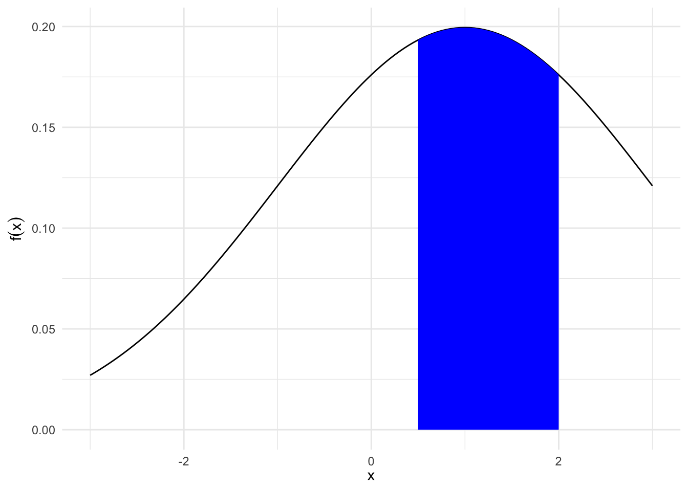
What is the area under the curve under \(f(x)\) between \(.5\) and \(2\)?
\[\int_{1/2}^{2} f(x)dx = F(2) - F(1/2)\]
Definition
\(X\) is a continuous random variable if there exists a nonnegative function defined for all \(x \in \Re\) having the property for any (measurable) set of real numbers \(B\),
\[ \begin{eqnarray} \Pr(X \in B) & = & \int_{B} f_X(x)dx \end{eqnarray} \]
- Non-negative meaning \(f(x)\) is never negative
- \(\Pr(X \in B)\): probability that \(X\) is is an element of \(B\)
- We’ll call \(f(\cdot)\) the probability density function (PDF) for \(X\)
The probability that the value of \(X\) falls within an interval is
\[\Pr (a \leq X \leq b) = \int_a^b f_X(x) dx\]
and can be interpreted as the area under the graph of the PDF. For any single value \(a\), we have \(\Pr (X = a) = \int_a^a f_X(x) dx = 0\). Note that to qualify as a PDF, a function \(f_X\) must be nonnegative, i.e. \(f_X(x) \geq 0\) for every \(x\), and must also have the normalization property
\[\int_{-\infty}^{\infty} f_X(x) dx = \Pr (-\infty \leq X \leq \infty) = 1\]
Example: Uniform Random Variable
\(X \sim \text{Uniform}(0,1)\)
\[ f_X(x) = \left\{ \begin{array}{ll} c & \quad \text{if } 0 \leq x \leq 1 \\ 0 & \quad \text{otherwise} \end{array} \right. \]
for some constant \(c\). The constant can be determined from the normalization property
\[1 = \int_{-\infty}^{\infty} f_X(x)dx = \int_0^1 c dx = c \int_0^1 dx = c\]
so that \(c=1\).
data_frame(x = seq(-.5, 1.5, by = .01),
           y = dunif(x)) %>%
  ggplot(aes(x, y)) +
  geom_step() +
  labs(x = expression(x),
       y = expression(f[X](x)))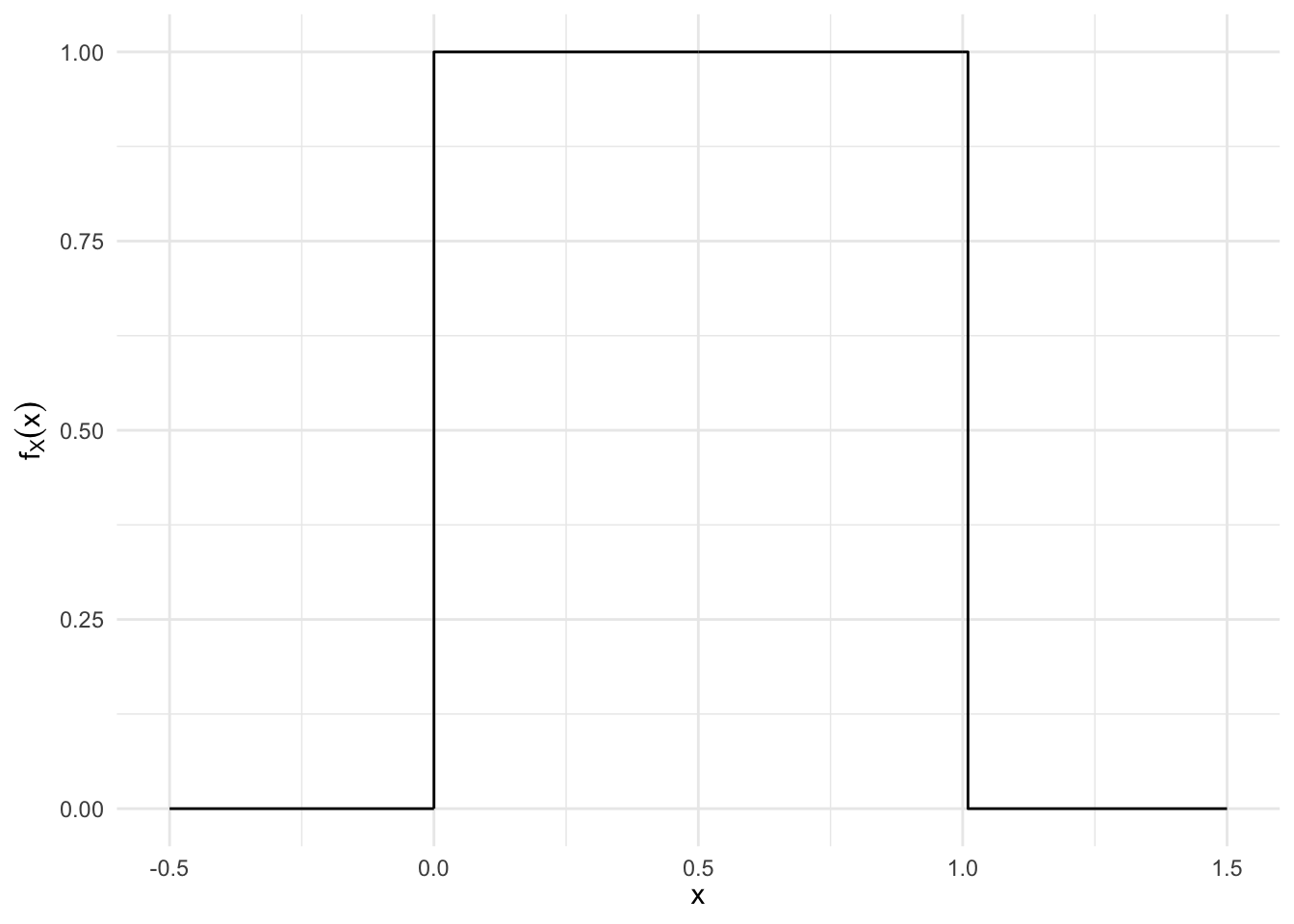
\[ \begin{eqnarray} \Pr(X \in [0.2, 0.5]) & = & \int_{0.2}^{0.5} 1 dx \nonumber \\ & = & X |^{0.5}_{0.2} \nonumber \\ & = & 0.5 - 0.2 \nonumber \\ & = & 0.3\nonumber \end{eqnarray} \]
\[ \begin{eqnarray} \Pr(X \in [0, 1] ) & = & \int_{0}^{1} 1 dx \nonumber \\ & = & X |^{1}_{0} \nonumber \\ & = & 1 - 0 \nonumber \\ & = & 1 \nonumber \end{eqnarray} \]
\[ \begin{eqnarray} \Pr(X \in [0.5, 0.5]) & = & \int_{0.5}^{0.5} 1dx \nonumber \\ & = & X|^{0.5}_{0.5} \nonumber \\ & = & 0.5 - 0.5 \nonumber \\ & = & 0 \nonumber \end{eqnarray} \]
\[ \begin{eqnarray} \Pr(X \in \{[0, 0.2]\cup[0.5, 1]\}) & = & \int_{0}^{0.2} 1dx + \int_{0.5}^{1} 1dx \nonumber \\ & = & X_{0}^{0.2} + X_{0.5}^{1} \nonumber \\ & = & 0.2 - 0 + 1 - 0.5 \nonumber \\ & = & 0.7 \nonumber \end{eqnarray} \]
More generally, the PDF of a uniform random variable has the form
\[ f_X(x) = \left\{ \begin{array}{ll} \frac{1}{b-a} & \quad \text{if } a \leq x \leq b \\ 0 & \quad \text{otherwise} \end{array} \right. \]
- To summarize
- \(\Pr(X = a) = 0\)
- \(\Pr(X \in (-\infty, \infty) ) = 1\)
- If \(F\) is antiderivative of \(f\), then \(\Pr(X \in [c,d]) = F(d) - F(c)\) (Fundamental theorem of calculus)
Expectation
The expected value of a continuous random variable \(X\) is defined as
\[\E[X] = \int_{-\infty}^{\infty} x f_X(x) dx\]
This is similar to the discrete case except instead of a summation operation, we use integration to calculate the expected value. If \(X\) is a continuous random variable with a given PDF, any real-valued function \(Y = g(X)\) is also a random variable. The mean of \(g(X)\) satisfies the expected value rule:
\[\E[g(X)] = \int_{-\infty}^{\infty} g(x) f_X(x) dx\]
- The \(n\)th moment is defined as \(\E[X^n]\), the expected value of the random variable \(X^n\)
- The variance, denoted by \(\Var(X)\) is defined as the expected value of the random variable \((X - \E[X])^2 = \E[X^2] - (\E[X])^2\)
Example: uniform random variable
Consider a uniform PDF over an interval \([a,b]\):
\[ \begin{align} \E[X] = \int_{-\infty}^{\infty} x f_X(x) dx &= \int_a^b x \times \frac{1}{b-a} dx \\ &= \frac{1}{b-a} \times \frac{1}{2}x^2 \Big|_a^b \\ &= \frac{1}{b-a} \times \frac{b^2 - a^2}{2} \\ &= \frac{a+b}{2} \end{align} \]
To obtain the variance, we first calculate the second moment. We have
\[ \begin{align} \E[X^2] = \int_a^b x^2 \times \frac{1}{b-a} dx &= \frac{1}{b-a} \int_a^b x^2 dx \\ &= \frac{1}{b-a} \times \frac{1}{3}x^3 \Big|_a^b \\ &= \frac{b^3 - a^3}{3(b-a)} \\ &= \frac{a^2 + ab + b^2}{3} \end{align} \]
Thus, the variance is
\[ \begin{align} \Var(X) = \E[X^2] - (\E[X])^2 = \frac{a^2 + ab + b^2}{3} - \left( \frac{a+b}{2} \right)^2 = \frac{(b-a)^2}{12} \end{align} \]
Exponential random variable
An exponential random variable has a PDF of the form
\[ f_X(x) = \left\{ \begin{array}{ll} \lambda e^{-\lambda x} & \quad \text{if } x \geq 0 \\ 0 & \quad \text{otherwise} \end{array} \right. \]
where \(\lambda\) is a positive parameter characterizing the PDF.
exp_pdf <- function(rate){
  data_frame(x = seq(0, 20, by = .05),
           pmf = dexp(x = x, rate = rate)) %>%
  ggplot(aes(x, pmf)) +
  geom_line() +
  labs(title = "Exponential PDF",
       subtitle = bquote(lambda == .(rate)),
       x = expression(x),
       y = expression(f[X] (x)))
}

exp_pdf(1) +
  exp_pdf(3) +
  exp_pdf(7)
\[\E[X] = \frac{1}{\lambda}, \quad \Var(X) = \frac{1}{\lambda^2}\]
It is frequently used to model phenomena of a continuous nature such as the time between arrivals (e.g. time between customers arriving at a restaraunt) and the distance between occurrences (e.g. distance between defects in a plate glass window). It is closely associated with the Poisson discrete random variable, which we will return to later.
Cumulative distribution function
- Probability density function (\(f\)) characterizes distribution of continuous random variable.
- Equivalently, cumulative distribution function characterizes continuous random variables
For a continuous random variable \(X\) define its cumulative distribution function (CDF) \(F_X(x)\) as,
\[ \begin{eqnarray} F_X(x) & = & P(X \leq x) = \int_{-\infty} ^{x} f_X(t) dt \end{eqnarray} \]
Example: uniform distribution
- Suppose \(X \sim Uniform(0,1)\), then
\[ \begin{eqnarray} F_X(x) & = & P(X\leq x) \\ & = & 0 \text{, if $x< 0$ } \\ & = & 1 \text{, if $x >1$ } \\ & = & x \text{, if $x \in [0,1]$} \end{eqnarray} \]
unif_pdf <- function(a, b){
  data_frame(x = seq(a - 1, b + 1, by = .01),
             pdf = dunif(x = x, min = a, max = b)) %>%
    ggplot(aes(x, pdf)) +
    geom_line() +
    labs(title = "Uniform PDF",
         subtitle = bquote(a == .(a) ~ b == .(b)),
         x = expression(x),
         y = expression(f[X] (x)))
}

unif_cdf <- function(a, b){
  data_frame(x = seq(a - 1, b + 1, by = .01),
             cdf = punif(q = x, min = a, max = b)) %>%
    ggplot(aes(x, cdf)) +
    geom_line() +
    labs(title = "Uniform CDF",
         subtitle = bquote(a == .(a) ~ b == .(b)),
         x = expression(x),
         y = expression(F[X] (x)))
}

unif_pdf(0, 1) +
  unif_cdf(0, 1)
Properties of CDFs
- \(F_X\) is monotonically nodecreasing – if \(x \leq y\), then \(F_X(x) \leq F_X(y)\)
- \(F_X(x)\) tends to \(0\) as \(x \rightarrow -\infty\), and to \(1\) as \(x \rightarrow \infty\)
- \(F_X(x)\) is a continuous function of \(x\)
If \(X\) is continuous, the PDF and CDF can be obtained from each other by integration or differentiation
\[F_X(x) = \int_{-\infty}^x f_X(t) dt, \quad f_X(x) = \frac{dF_X}{dx} (x)\]
Normal random variables
Suppose \(X\) is a random variable with \(X \in \Re\) and density
\[ \begin{eqnarray} f(x) & = & \frac{1}{\sqrt{2\pi \sigma^2}}\exp\left(-\frac{(x - \mu)^2}{2\sigma^2}\right) \nonumber \end{eqnarray} \]
where \(\mu\) and \(\sigma\) are two scalar parameters characterizing the PDF, with \(\sigma\) assumed positive. Then \(X\) is a normally distributed random variable with parameters \(\mu\) and \(\sigma^2\).
norm_pdf <- function(mu, sigma){
  data_frame(x = seq(-5, 5, by = .01),
             pdf = dnorm(x = x, mean = mu, sd = sigma)) %>%
    ggplot(aes(x, pdf)) +
    geom_line() +
    labs(title = "Normal PDF",
         subtitle = bquote(mu == .(mu) ~ sigma^2 == .(sigma^2)),
         x = expression(x),
         y = expression(f[X] (x)))
}

norm_cdf <- function(mu, sigma){
  data_frame(x = seq(-5, 5, by = .01),
             cdf = pnorm(q = x, mean = mu, sd = sigma)) %>%
    ggplot(aes(x, cdf)) +
    geom_line() +
    labs(title = "Normal CDF",
         subtitle = bquote(mu == .(mu) ~ sigma^2 == .(sigma^2)),
         x = expression(x),
         y = expression(f[X] (x)))
}

norm_pdf(0, 1) +
  norm_cdf(0, 1)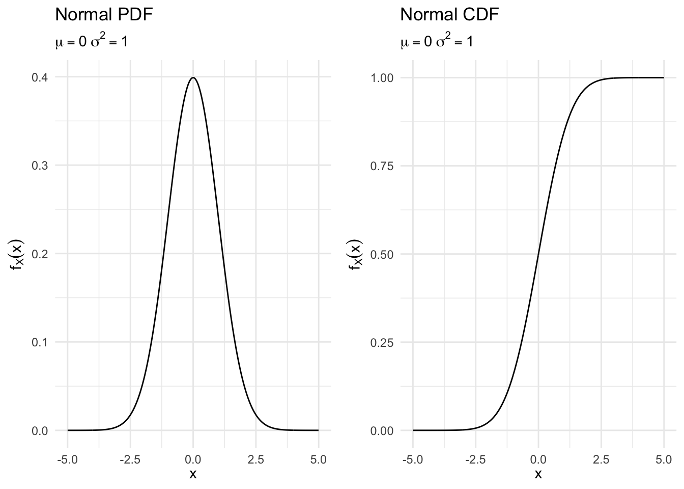
Equivalently, we’ll write
\[ \begin{eqnarray} X & \sim & \text{Normal}(\mu, \sigma^2) \nonumber \end{eqnarray} \]
Expected value/variance of normal distribution
\(Z\) is a standard normal distribution if
\[ \begin{eqnarray} Z & \sim & \text{Normal}(0,1) \nonumber \end{eqnarray} \]
We’ll call the cumulative distribution function of \(Z\),
\[ \begin{eqnarray} F_{Z}(x) & = & \frac{1}{\sqrt{2\pi} }\int_{-\infty}^{x} \exp(-z^2/2) dz \end{eqnarray} \]
Suppose \(Z \sim \text{Normal}(0,1)\)
- \(Y = 2Z + 6\)
\(Y \sim \text{Normal}(6, 4)\)
data_frame(x = seq(-5, 15, by = .05),
           Z = dnorm(x),
           Y = dnorm(x, mean = 6, sd = 2)) %>%
  gather(norm, val, -x) %>%
  ggplot(aes(x, val, color = norm)) +
  geom_line() +
  scale_color_brewer(type = "qual") +
  labs(x = NULL,
       y = "Density height",
       color = NULL) +
  theme(legend.position = "bottom")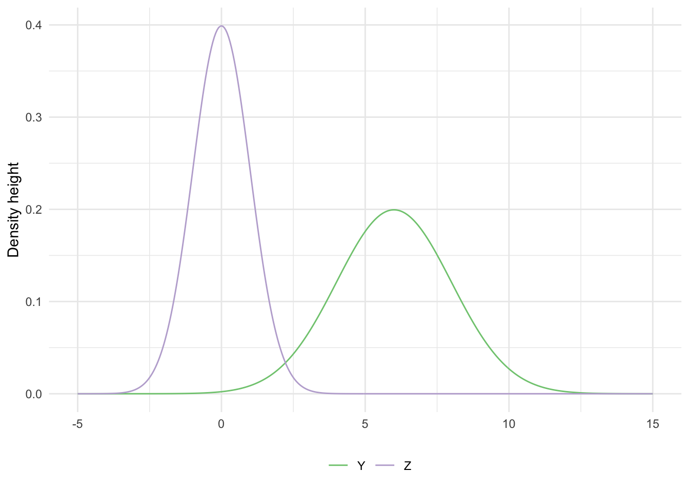
Scale/Location: If \(Z \sim N(0,1)\), then \(X = aZ + b\) is,
\[ \begin{eqnarray} X & \sim & \text{Normal} (b, a^2) \nonumber \end{eqnarray} \]
Assume we know:
\[ \begin{eqnarray} \E[Z] & = & 0 \\ \Var(Z) & = & 1 \end{eqnarray} \]
This implies that, for \(Y \sim \text{Normal}(\mu, \sigma^2)\)
\[ \begin{eqnarray} \E[Y] & = & \E[\sigma Z + \mu] \\ & = & \sigma \E[Z] + \mu \nonumber \\ & = & \mu \nonumber \\ \Var(Y) & = & \Var(\sigma Z + \mu) \\ & = & \sigma^2 \Var(Z) + \Var(\mu) \\ & = & \sigma^2 + 0 \\ & =& \sigma^2 \end{eqnarray} \]
This illustrates a key property of normal random variables. If \(X\) is a normal random variable with mean \(\mu\) and variance \(\sigma^2\), and if \(a \neq 0, b\) are scalars, then the random variable
\[Y = aX + b\]
is also normal, with mean and variance
\[\E[Y] = a\mu + b, \quad \Var(Y) = a^2 \sigma^2\]
Why rely on the standard normal distribution
- Normal distribution is commonly used in statistical analysis
- Many random variables can be approximated with the normal distribution
- Standardizing this makes it easier to make comparisons across variables with different ranges/variances
- Example - GRE scores
- Verbal and quant scores have different variability
- Cannot easily determine if a 159 on the verbal is better or worse than a 159 on the quant
- The standard normal distribution is unitless, so any random variable can be compared with another random variable
- Saves time on the calculus
- Don’t need to recalculate the integral when calculating cumulative probability based on the unique \(\mu\) and \(\sigma^2\)
- Instead, do this once and store the info in a lookup table
- Made calculating probabilities (relatively) easy before computers
Example: Support for President Obama
Suppose we are interested in modeling presidential approval.
- Let \(Y\) represent random variable: proportion of population who “approves job president is doing”
- Individual responses (that constitute proportion) are independent and identically distributed (sufficient, not necessary) and we take the average of those individual responses
- Observe many responses (\(N\rightarrow \infty\))
- Then (by Central Limit Theorm) \(Y\) is Normally distributed, or
\[ \begin{eqnarray} Y & \sim & \text{Normal}(\mu, \sigma^2) \\ f_Y(y) & = & \frac{1}{\sqrt{2\pi \sigma^2}} \exp\left(-\frac{(y-\mu)^2}{2\sigma^2} \right) \end{eqnarray} \]
- Suppose \(\mu = 0.39\) and \(\sigma^2 = 0.0025\)
- \(\Pr(Y\geq 0.45)\) (What is the probability it isn’t that bad?) ?
\[ \begin{eqnarray} \Pr(Y \geq 0.45) & = & 1 - \Pr(Y \leq 0.45 ) \\ & = & 1 - \Pr(0.05 Z + 0.39 \leq 0.45) \\ & = & 1 - \Pr(Z \leq \frac{0.45-0.39 }{0.05} ) \\ & = & 1 - \frac{1}{\sqrt{2\pi} } \int_{-\infty}^{6/5} \exp(-z^2/2) dz \\ & = & 1 - F_{Z} (\frac{6}{5} ) \\ & = & 0.1150697 \end{eqnarray} \]
Conditioning
We can condition a random variable on an event or on another random variable, and define the concepts of conditional PDF and conditional expectation.
Conditioning a random variable on an event
The conditional PDF of a continuous random variable \(X\), given an event \(A\) with \(\Pr (A) > 0\), is defined as a nonnegative function \(f_{X|A}\) that satisfies
\[\Pr (X \in B | A) = \int_B f_{X|A}(x) dx\]
for any subset \(B\) of the real line. By letting \(B\) be the entire real line, we obtain the normalization property
\[\int_{-\infty}^{\infty} f_{X|A} (x) dx = 1\]
so that \(f_{X|A}\) is a legitimate PDF. Based on the definition of conditional probabilities, when we condition on an event of the form \({X \in A}\) with \(\Pr (X \in A) > 0\) we get
\[\Pr (X \in B | X \in A) = \frac{\Pr (X \in B, X \in A)}{\Pr (X \in A)} = \frac{\int_{A \cap B} f_X(x) dx}{\Pr (X \in A)}\]
Therefore the conditional PDF is
\[ f_{X | X \in A} (x) = \left\{ \begin{array}{ll} \frac{f_X (x)}{\Pr (X \in A)} & \quad \text{if } x \in A \\ 0 & \quad \text{otherwise} \end{array} \right. \]
Within the conditioning set, the conditional PDF has exactly the same shape as the unconditional one, except that it is scaled by the constant factor \(1 / \Pr (X \in A)\), so that \(f_{X | \{X \in A\}}\) integrates to 1. Thus, the conditional PDF is similar to an ordinary PDF, except that it refers to a new universe in which the event \(\{ X \in A \}\) is known to have occurred.
data_frame(x = seq(-3, 3, by = .01),
           pdf = dnorm(x = x),
           pdf_cond = ifelse(x > -1 & x < 1, pdf / (pnorm(1) - pnorm(-1)), 0)) %>%
  gather(pdf, value, -x) %>%
  ggplot(aes(x, value, color = pdf)) +
  geom_line() +
  scale_color_brewer(type = "qual", labels = c(expression(f[X](x)), expression(f[X*"|"*X %in% A](x)))) +
  labs(title = "Standard normal random variable",
       x = expression(X),
       y = "PDF",
       color = NULL) +
  theme(legend.position = "bottom")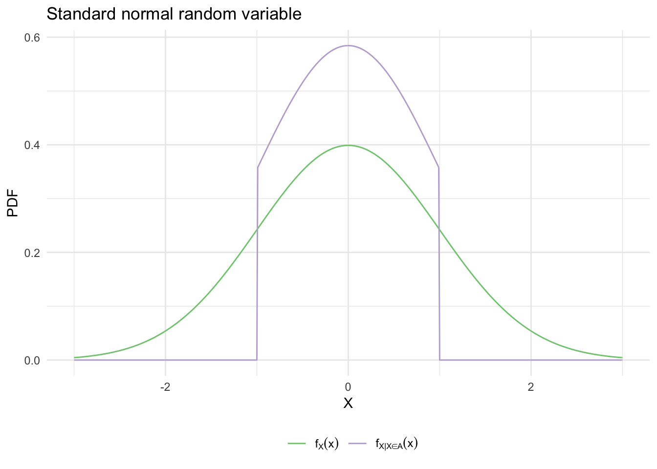
Example: Exponential random variable
The time \(T\) until a new light bulb burns out is an exponential random variable with parameter \(\lambda\). Ariadne turns on the light, leaves the room, and when she returns, \(t\) time units later, finds that the light bulb is still on, which corresponds to the event \(A = \{ T > t \}\). Let \(X\) be the additional time until the light bulb burns out. What is the conditional PDF of \(X\), given the event \(A\)?
We have, for \(x \geq 0\),
\[ \begin{align} \Pr (X > x | A) &= \Pr (T > t + x | T > t) \\ &= \frac{\Pr (T > t + x )\cap \Pr(T > t)}{\Pr( T >t)} \\ &= \frac{\Pr (T > t + x)}{\Pr (T > t)} \\ &= \frac{1 - \lambda e^{-\lambda(t + x)}}{1 - \lambda e^{-\lambda t}} \\ &= \frac{ e^{-\lambda(t + x)}}{ e^{-\lambda t}} \\ &= e^{-\lambda x} \end{align} \]
where we use the CDF of the exponential random variable. Thus, the conditional PDF of \(X\) is exponential with parameter \(\lambda\), regardless of the time \(t\) that has elapsed between lighting the bulb and Ariadne’s arrival (known as the memorylessness property of the exponential).
Practice working with continuous random variables in R
Weather forecasting
According to British weather forecasters, the average monthly rainfall in London during the month of June is \(\mu = 2.09\) inches. Assume the monthly precipitation is a normally-distributed random variable with a standard deviation of \(\sigma = 0.48\) inches.
What is the probability that London will have between 1.5 and 2.5 inches of precipitation next June?
Click for the solution
\[\Pr (1.5 \leq x \leq 2.5) = \Pr (-1.23 \leq z \leq 0.85) = 0.694\]
pnorm(q = 2.5, mean = 2.09, sd = 0.48) - pnorm(q = 1.5, mean = 2.09, sd = 0.48)## [1] 0.694What is the probability that London will have 1 inch or less of precipitation?
Click for the solution
\[\Pr (x \leq 1) = \Pr (z \leq -2.27) = 0.012\]
pnorm(q = 1, mean = 2.09, sd = 0.48)## [1] 0.0116Booking travel (redux)
Book4Less.com is an online travel website that offers competitive prices on airline and hotel bookings. During a typical weekday, the website averages 10 visits per minute.
If the Poisson arrival rate is 10 visitors per minute, what is the mean of the associated exponential probility density function? What is the rate parameter \(\lambda\)?
Click for the solution
If the mean Poisson arrival rate is 10 visitors per minute (every sixty seconds), then the average time between passenger visitors is exponentially-distributed with a mean of 6 seconds.
\[\E[X] = \frac{1}{\lambda} \equiv \mu\]
\[\lambda = \frac{1}{\mu} = \frac{1}{6}\]
What is the exponential PDF and CDF?
Click for the solution
\[ \begin{align} f_X(x) &= \lambda e^{-\lambda x} = \frac{1}{6} e^{- \frac{1}{6}x} \\ F_X(x) &= 1 - e^{-\lambda x} = 1 - e^{-\frac{1}{6} x}, \quad \text{for } x > 0 \end{align} \]
If the internet server experiences a brief power failure of 18 seconds duration during which time people would be denied access to the website, what is the probability that no one attempted to visit the Book4Less.com website anyway and thus no business was lost during the down-time? Use the exponential framework to answer this question.
Click for the solution
\[\Pr (x \geq 18) = 1 - \Pr (X \leq 18) = 1 - (1 - e^{-\frac{18}{6}}) = e^{-\frac{18}{6}} = 0.05\]
1 - pexp(q = 18, rate = 1/6)## [1] 0.0498Answer the previous question using the Poisson probability approach. Confirm that the answer is equal to that above.
Click for the solution
Since we are told that there is an average of 10 visitors per minute, or 10 visitors per 60 seconds, we need to convert this parameter: \(\mu = \frac{10 \text{ visitors}}{60 \text{ seconds}} = \frac{3 \text{ visitors}}{18 \text{ seconds}}\).
Recall that the Poisson probability function is
\[ \begin{align} f_X(x | \lambda) &= e^{-\lambda} \frac{\lambda^{x}}{x!}, \quad x = 0,1,2,\ldots \\ f_X(x = 0 | \lambda = 3) &= e^{-3} \frac{3^{0}}{0!} \\ &= e^{-3} \\ &= 0.05 \end{align} \]
dpois(x = 0, lambda = 3)## [1] 0.0498If the interval of time (or distance) between occurrences is distributed exponentially, then the number of occurrences in that interval must be Poisson-distributed. The two distributions are interrelated. See here for a more in-depth explanation.
Acknowledgements
- Material drawn from Introduction to Probability (2nd edition) by Bertsekas and Tsitsiklis
Session Info
devtools::session_info()## Session info -------------------------------------------------------------## setting value
## version R version 3.5.1 (2018-07-02)
## system x86_64, darwin15.6.0
## ui X11
## language (EN)
## collate en_US.UTF-8
## tz America/Chicago
## date 2018-11-06## Packages -----------------------------------------------------------------## package * version date source
## assertthat 0.2.0 2017-04-11 CRAN (R 3.5.0)
## backports 1.1.2 2017-12-13 CRAN (R 3.5.0)
## base * 3.5.1 2018-07-05 local
## bindr 0.1.1 2018-03-13 CRAN (R 3.5.0)
## bindrcpp 0.2.2 2018-03-29 CRAN (R 3.5.0)
## broom * 0.5.0 2018-07-17 CRAN (R 3.5.0)
## cellranger 1.1.0 2016-07-27 CRAN (R 3.5.0)
## cli 1.0.0 2017-11-05 CRAN (R 3.5.0)
## colorspace 1.3-2 2016-12-14 CRAN (R 3.5.0)
## compiler 3.5.1 2018-07-05 local
## crayon 1.3.4 2017-09-16 CRAN (R 3.5.0)
## datasets * 3.5.1 2018-07-05 local
## devtools 1.13.6 2018-06-27 CRAN (R 3.5.0)
## digest 0.6.18 2018-10-10 cran (@0.6.18)
## dplyr * 0.7.6 2018-06-29 cran (@0.7.6)
## evaluate 0.11 2018-07-17 CRAN (R 3.5.0)
## forcats * 0.3.0 2018-02-19 CRAN (R 3.5.0)
## ggplot2 * 3.1.0 2018-10-25 cran (@3.1.0)
## glue 1.3.0 2018-07-17 CRAN (R 3.5.0)
## graphics * 3.5.1 2018-07-05 local
## grDevices * 3.5.1 2018-07-05 local
## grid 3.5.1 2018-07-05 local
## gtable 0.2.0 2016-02-26 CRAN (R 3.5.0)
## haven 1.1.2 2018-06-27 CRAN (R 3.5.0)
## hms 0.4.2 2018-03-10 CRAN (R 3.5.0)
## htmltools 0.3.6 2017-04-28 CRAN (R 3.5.0)
## httr 1.3.1 2017-08-20 CRAN (R 3.5.0)
## jsonlite 1.5 2017-06-01 CRAN (R 3.5.0)
## knitr 1.20 2018-02-20 CRAN (R 3.5.0)
## lattice 0.20-35 2017-03-25 CRAN (R 3.5.1)
## lazyeval 0.2.1 2017-10-29 CRAN (R 3.5.0)
## lubridate 1.7.4 2018-04-11 CRAN (R 3.5.0)
## magrittr 1.5 2014-11-22 CRAN (R 3.5.0)
## memoise 1.1.0 2017-04-21 CRAN (R 3.5.0)
## methods * 3.5.1 2018-07-05 local
## modelr 0.1.2 2018-05-11 CRAN (R 3.5.0)
## munsell 0.5.0 2018-06-12 CRAN (R 3.5.0)
## nlme 3.1-137 2018-04-07 CRAN (R 3.5.1)
## patchwork * 0.0.1 2018-09-06 Github (thomasp85/patchwork@7fb35b1)
## pillar 1.3.0 2018-07-14 CRAN (R 3.5.0)
## pkgconfig 2.0.2 2018-08-16 CRAN (R 3.5.1)
## plyr 1.8.4 2016-06-08 CRAN (R 3.5.0)
## purrr * 0.2.5 2018-05-29 CRAN (R 3.5.0)
## R6 2.2.2 2017-06-17 CRAN (R 3.5.0)
## Rcpp 0.12.19 2018-10-01 cran (@0.12.19)
## readr * 1.1.1 2017-05-16 CRAN (R 3.5.0)
## readxl 1.1.0 2018-04-20 CRAN (R 3.5.0)
## rlang 0.3.0.1 2018-10-25 cran (@0.3.0.1)
## rmarkdown 1.10 2018-06-11 CRAN (R 3.5.0)
## rprojroot 1.3-2 2018-01-03 CRAN (R 3.5.0)
## rstudioapi 0.7 2017-09-07 CRAN (R 3.5.0)
## rvest 0.3.2 2016-06-17 CRAN (R 3.5.0)
## scales 1.0.0 2018-08-09 CRAN (R 3.5.0)
## stats * 3.5.1 2018-07-05 local
## stringi 1.2.4 2018-07-20 CRAN (R 3.5.0)
## stringr * 1.3.1 2018-05-10 CRAN (R 3.5.0)
## tibble * 1.4.2 2018-01-22 CRAN (R 3.5.0)
## tidyr * 0.8.1 2018-05-18 CRAN (R 3.5.0)
## tidyselect 0.2.4 2018-02-26 CRAN (R 3.5.0)
## tidyverse * 1.2.1 2017-11-14 CRAN (R 3.5.0)
## tools 3.5.1 2018-07-05 local
## utils * 3.5.1 2018-07-05 local
## withr 2.1.2 2018-03-15 CRAN (R 3.5.0)
## xml2 1.2.0 2018-01-24 CRAN (R 3.5.0)
## yaml 2.2.0 2018-07-25 CRAN (R 3.5.0)This work is licensed under the CC BY-NC 4.0 Creative Commons License.