library(tidyverse)
library(broom)
library(patchwork)

options(digits = 3)
set.seed(1234)
theme_set(theme_minimal())

\[\newcommand{\E}{\mathrm{E}} \newcommand{\Var}{\mathrm{Var}} \newcommand{\Cov}{\mathrm{Cov}}\]

Basic concepts

Random variable - real-valued function of the outcome of an experiment
Function of a random variables - defines another random variable
Associated each random variable with “averages” of interest, such as the mean or the variance
A random variable can be conditioned on an event or on another random variable
Independence of a random variable from an event or from another random variable

Random variable

A random process or variable with a numerical outcome
More formally, it is a random variable \(X\) that is a function of the sample space
- Number of incumbents who win
- An indicator whether a country defaults on a loan (1 if a default, 0 otherwise)
- Number of casualties in a war (rather than all possible outcomes)
\[ \begin{eqnarray} X:\text{Sample Space} \rightarrow \mathcal{R} \end{eqnarray} \]

Examples

Treatment assignment:
- Suppose we have \(3\) units, flipping fair coin (\(\frac{1}{2}\)) to assign each unit
- Assign to \(T=\)Treatment or \(C=\)control
- \(X\) = Number of units received treatment
- Defining the function
  \[ \begin{equation} X = \left \{ \begin{array} {ll} 0 \text{ if } (C, C, C) \\ 1 \text{ if } (T, C, C) \text{ or } (C, T, C) \text{ or } (C, C, T) \\ 2 \text{ if } (T, T, C) \text{ or } (T, C, T) \text{ or } (C, T, T) \\ 3 \text{ if } (T, T, T) \end{array} \right. \end{equation} \]
- In other words:
  \[ \begin{eqnarray} X( (C, C, C) ) & = & 0 \\ X( (T, C, C)) & = & 1 \\ X((T, C, T)) & = & 2 \\ X((T, T, T)) & = & 3 \end{eqnarray} \]
\(X\) = Number of Calls into congressional office in some period \(p\)
- \(X(c) = c\)
Outcome of Election
- Define \(v\) as the proportion of vote the candidate receives
- Define \(X = 1\) if \(v>0.50\)
- Define \(X = 0\) if \(v<0.50\)
- For example, if \(v = 0.48\), then \(X(v) = 0\)
An indicator whether a country defaults on a loan (1 if a default, 0 otherwise)
Not all are experimental - most are observational

Discrete random variables

A random variable with a finite or countably infinite range
A random variable with an uncountably infinite number of values is continuous

Probability mass functions

Probability of the values that it can take
Probability mass function (PMF)
Go back to our experiment example – probability comes from probability of outcomes
\(P(C, T, C) = P(C)P(T)P(C) = \frac{1}{2}\frac{1}{2}\frac{1}{2} = \frac{1}{8}\)
This applies to all outcomes
\[ \begin{eqnarray} p(X = 0) & = & P(C, C, C) = \frac{1}{8}\\ p(X = 1) & = & P(T, C, C) + P(C, T, C) + P(C, C, T) = \frac{3}{8} \\ p(X = 2) & = & P(T, T, C) + P(T, C, T) + P(C, T, T) = \frac{3}{8} \\ p(X = 3) & = & P(T, T, T) = \frac{1}{8} \end{eqnarray} \]
\(p(X = a) = 0\), for all \(a \notin (0, 1, 2, 3)\)

pmf <- data_frame(x = 0:3,
           y = c(1/8, 3/8, 3/8, 1/8))

pmf %>%
  ggplot(aes(x, y)) +
  geom_col() +
  labs(title = "Probability Mass Function",
       x = "Number of treated",
       y = "Probability")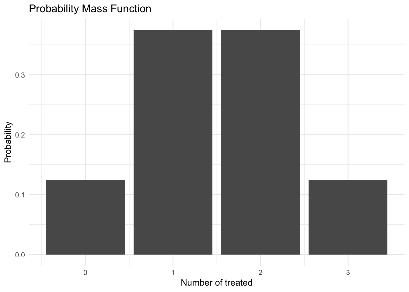

Probability Mass Function: For a discrete random variable \(X\), define the probability mass function \(p_X(x)\) as
\[ \begin{eqnarray} p_X(x) & = & P(X = x) \end{eqnarray} \]
Use upper-case letters to denote random variables, use lower-case letters to denote real numbers such as the numerical values of a random variable
Note that

\[\sum_x p_{X}(x) = 1\]
- \(x\) ranges over all possible values of \(X\)
- Makes sense - probability must sum to 1
Can also add probabilities for smaller sets \(S\) of possible values of \(XS\)
\[\Pr(X \in S) = \sum_{x \in S} p_X (x)\]
For example, if \(X\) is the number of heads obtained in two independent tosses of a fair coin, the probability of at least one head is

\[\Pr (X > 0) = \sum_{x=1}^2 p_X (x) = \frac{1}{2} + \frac{1}{4} = \frac{3}{4}\]
To calculate the PMF of a random variable \(X\)
- For each possible value \(x\) of \(X\)
  1. Collect all possible outcomes that give rise to the event \(\{ X=x \}\)
  2. Add their probabilities to obtain \(p_X (x)\)

Famous discrete random variables

Bernoulli

Suppose \(X\) is a random variable, with \(X \in \{0, 1\}\) and \(P(X = 1) = \pi\). Then we will say that \(X\) is Bernoulli random variable,

\[ \begin{eqnarray} p_X(k) & = & \pi^{k} (1- \pi)^{1 - k} \nonumber \end{eqnarray} \]

for \(k \in \{0,1\}\) and \(p(k) = 0\) otherwise.
- \(\pi\) does not refer to \(3.14159\) in this instance, it is a variable
We will (equivalently) say that

\[ \begin{eqnarray} Y & \sim & \text{Bernoulli}(\pi) \nonumber \end{eqnarray} \]
Suppose we flip a fair coin and \(Y = 1\) if the outcome is Heads.

\[ \begin{eqnarray} Y & \sim & \text{Bernoulli}(1/2) \nonumber \\ p(1) & = & (1/2)^{1} (1- 1/2)^{ 1- 1} = 1/2 \nonumber \\ p(0) & = & (1/2)^{0} (1- 1/2)^{1 - 0} = (1- 1/2) \nonumber \end{eqnarray} \]

bernouli_plot <- function(p){
  data_frame(x = 0:1,
             p = dbinom(x = x, size = 1, prob = p)) %>%
    mutate(x = factor(x)) %>%
    ggplot(aes(x, p)) +
    geom_col() +
    labs(title = "Bernouli PMF",
         subtitle = bquote(pi == .(p)),
         x = expression(x),
         y = expression(P[X] (k)))
}
bernouli_plot(.5) +
  bernouli_plot(.7) +
  bernouli_plot(.3)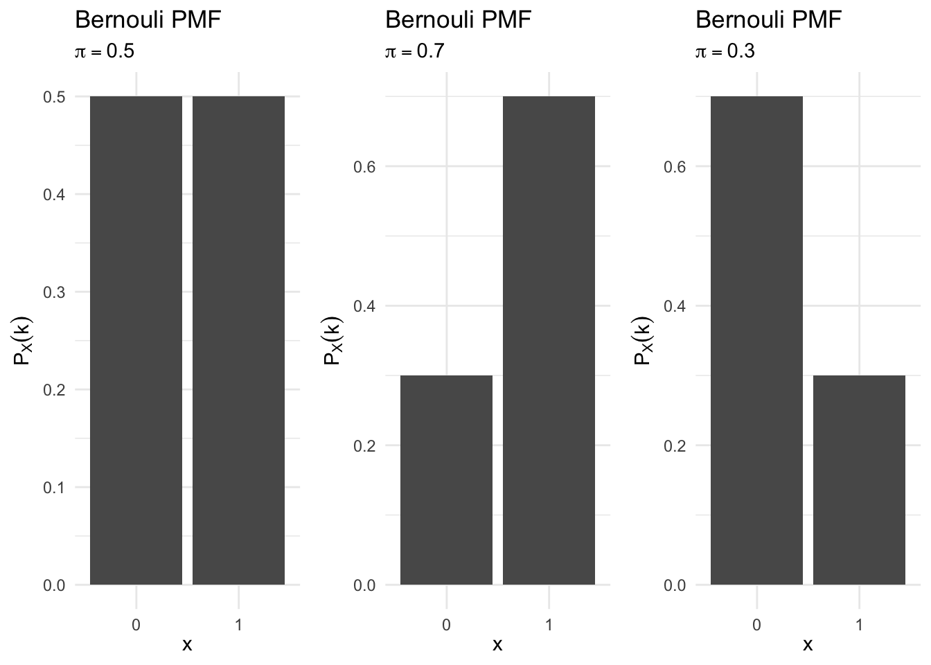

Other examples
- Person is healthy or sick
- Person votes or does not vote

Binomial

A model to count the number of successes across \(N\) trials
Suppose \(X\) is a random variable that counts the number of successes in \(N\) independent and identically distributed Bernoulli trials. Then \(X\) is a Binomial random variable,

\[ \begin{eqnarray} p_X(k) & = & {{N}\choose{k}}\pi^{k} (1- \pi)^{n-k} \nonumber \end{eqnarray} \]

for \(k \in \{0, 1, 2, \ldots, N\}\) and \(p(k) = 0\) otherwise, and \(\binom{N}{k} = \frac{N!}{(N-k)! k!}\). Equivalently,

\[ \begin{eqnarray} Y & \sim & \text{Binomial}(N, \pi) \nonumber \end{eqnarray} \]

Example

binomial_plot <- function(n, p){
  data_frame(x = 0:n,
             p = dbinom(x = x, size = n, prob = p)) %>%
    mutate(x = factor(x)) %>%
    ggplot(aes(x, p)) +
    geom_col() +
    labs(title = "Binomial PMF",
         subtitle = bquote(n == .(n) ~ p == .(p)),
         x = expression(x),
         y = expression(P[X] (k)))
}
binomial_plot(10, .5)

binomial_plot(10, .3)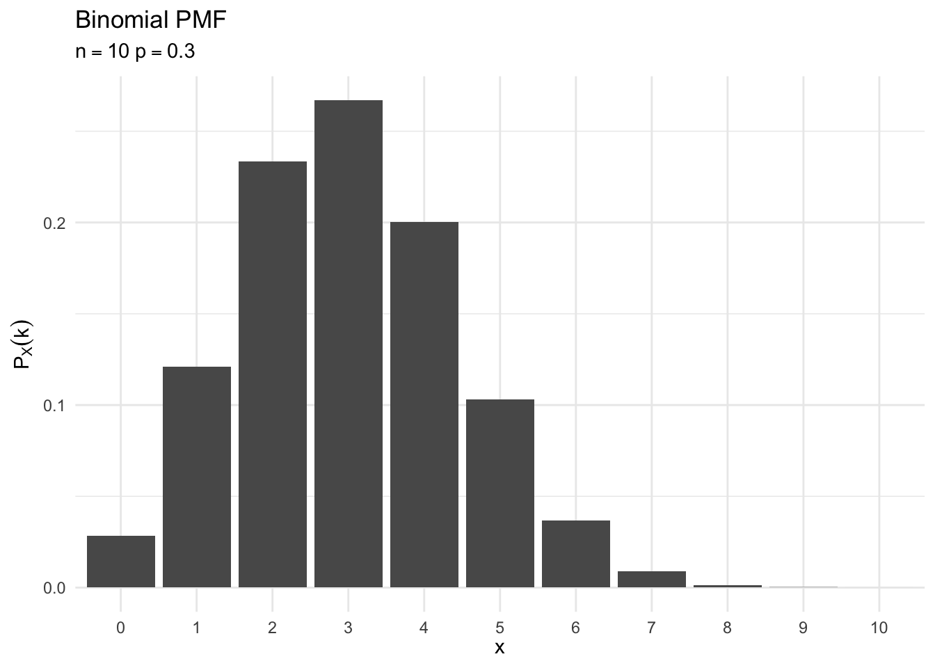

binomial_plot(100, .2)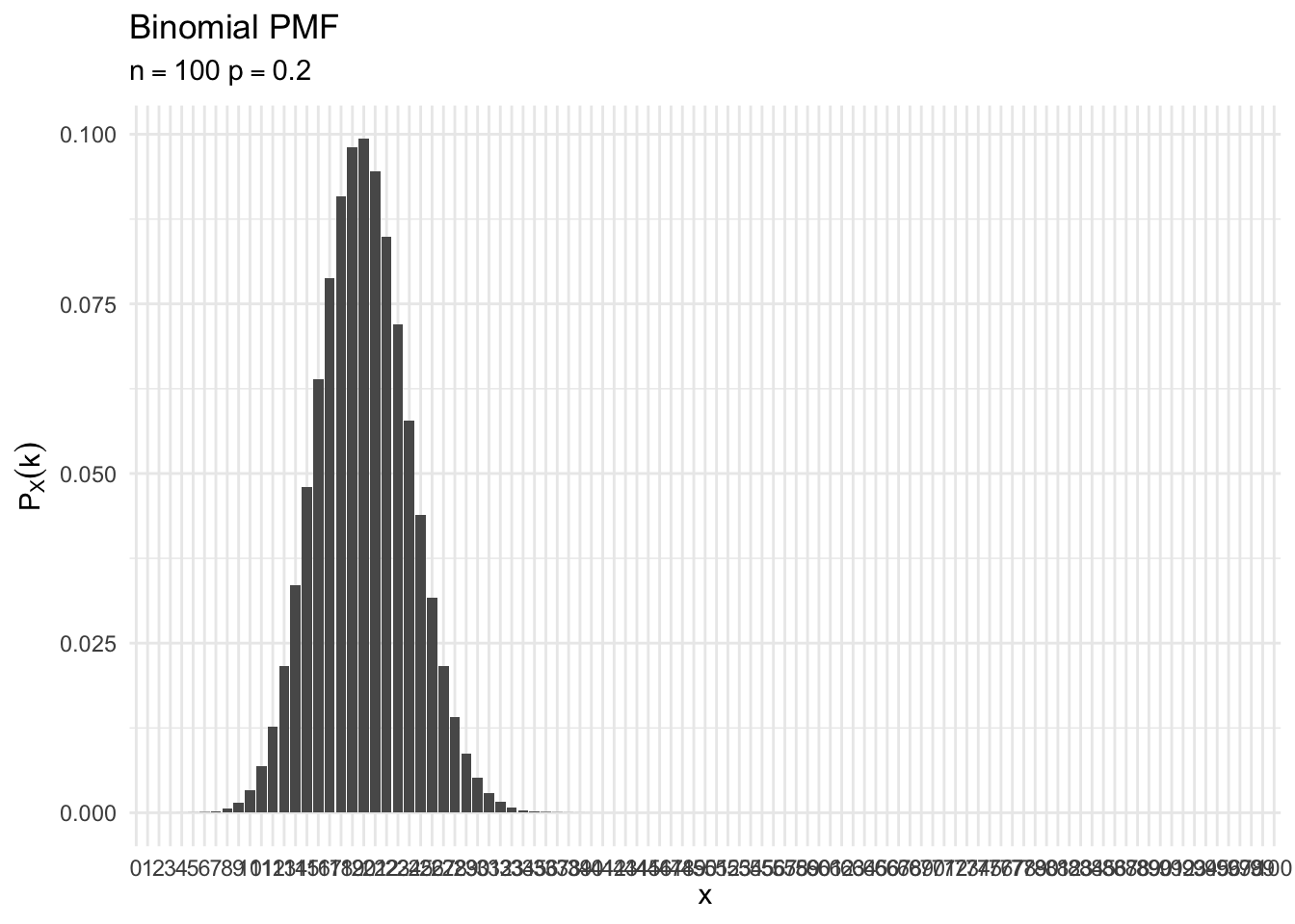

binomial_plot(100, .8)

Recall our experiment example:
- \(P(T) = P(C) = 1/2\)
- \(Z =\) number of units assigned to treatment
\[ \begin{eqnarray} Z & \sim & \text{Binomial}(1/2)\\ p(0) & = & {{3}\choose{0}} (1/2)^{0} (1- 1/2)^{3-0} = 1 \times \frac{1}{8}\\ p(1) & = & {{3}\choose{1}} (1/2)^{1} (1 - 1/2)^{2} = 3 \times \frac{1}{8} \\ p(2) & = & {{3}\choose{2}} (1/2)^{2} (1- 1/2)^1 = 3 \times \frac{1}{8} \\ p(3) & = & {{3}\choose{3}} (1/2)^{3} (1 - 1/2)^{0} = 1 \times \frac{1}{8} \end{eqnarray} \]

Geometric

A model to count the number of trials of a Bernouli outcome before success occurs the first time
Suppose \(X\) is a random variable that counts the number of tosses needed for a head to come up the first time. Its PMF is
\[ \begin{eqnarray} p_X(k) & = & (1 - p)^{k-1}p, \quad k = 1, 2, \ldots \end{eqnarray} \]
- \((1 - p)^{k-1}p\) is the probability of the sequence consisting of \(k-1\) successive trials followed by a head. This is a valid PMF because
\[ \begin{align} \sum_{k=1}^{\infty} p_X(k) &= \sum_{k=1}^{\infty} (1 - p)^{k-1}p \\ &= p \sum_{k=1}^{\infty} (1 - p)^{k-1} \\& = p \times \frac{1}{1 - (1-p)} \\ &= 1 \end{align} \]

geometric_plot <- function(p){
  data_frame(x = 0:20,
             p = dgeom(x = x, prob = p)) %>%
    mutate(x = factor(x + 1)) %>%
    ggplot(aes(x, p)) +
    geom_col() +
    labs(title = "Geometric PMF",
         subtitle = bquote(p == .(p)),
         x = expression(x),
         y = expression(P[X] (k)))
}

geometric_plot(.5)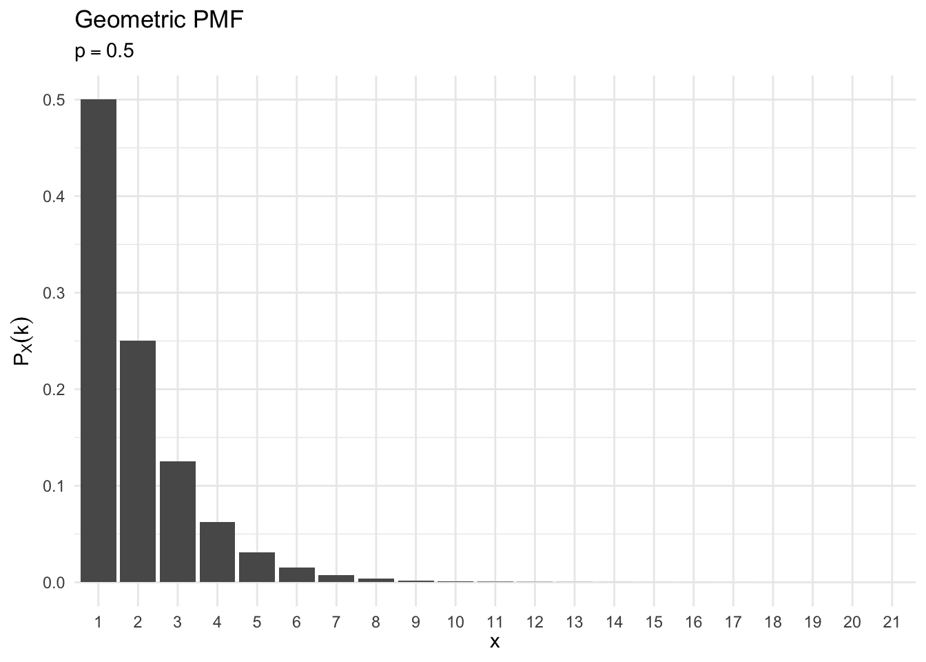

geometric_plot(.7)

geometric_plot(.2)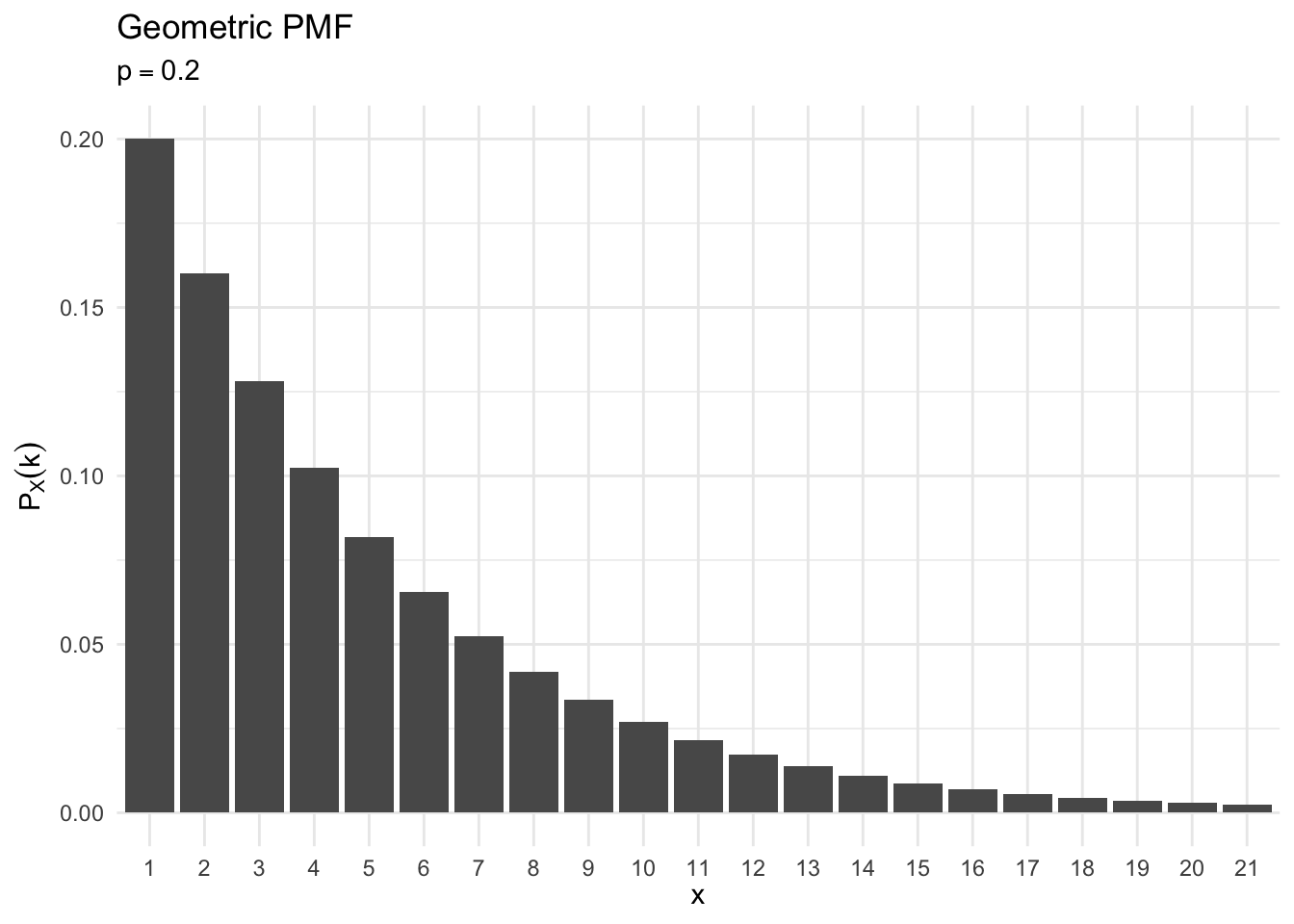

Examples
- Number of attempts before passing a test
- Finding a missing item in a search

Poisson

Often interested in counting number of events that occur:
- Number of wars started
- Number of speeches made
- Number of bribes offered
- Number of people waiting for license
Generally referred to as event counts
Suppose \(X\) is a random variable that takes on values \(X \in \{0, 1, 2, \ldots, \}\) and that \(\Pr(X = k) = p_X(k)\) is,

\[ \begin{eqnarray} p_X(k) & = & e^{-\lambda} \frac{\lambda^{k}}{k!}, \quad k = 0,1,2,\ldots \end{eqnarray} \]

for \(k \in \{0, 1, \ldots, \}\) and \(0\) otherwise.

for \(k \in \{0, 1, \ldots, \}\) and \(0\) otherwise. Then we will say that \(X\) follows a Poisson distribution with rate parameter \(\lambda\)

\[ \begin{eqnarray} X & \sim & \text{Poisson}(\lambda) \nonumber \end{eqnarray} \]

poisson_plot <- function(lambda, max_n = 10){
  data_frame(x = 0:max_n,
             p = dpois(x = x, lambda = lambda)) %>%
    mutate(x = factor(x)) %>%
    ggplot(aes(x, p)) +
    geom_col() +
    labs(title = "Poisson PMF",
         subtitle = bquote(lambda == .(lambda)),
         x = expression(x),
         y = expression(P[X] (k)))
}
poisson_plot(2)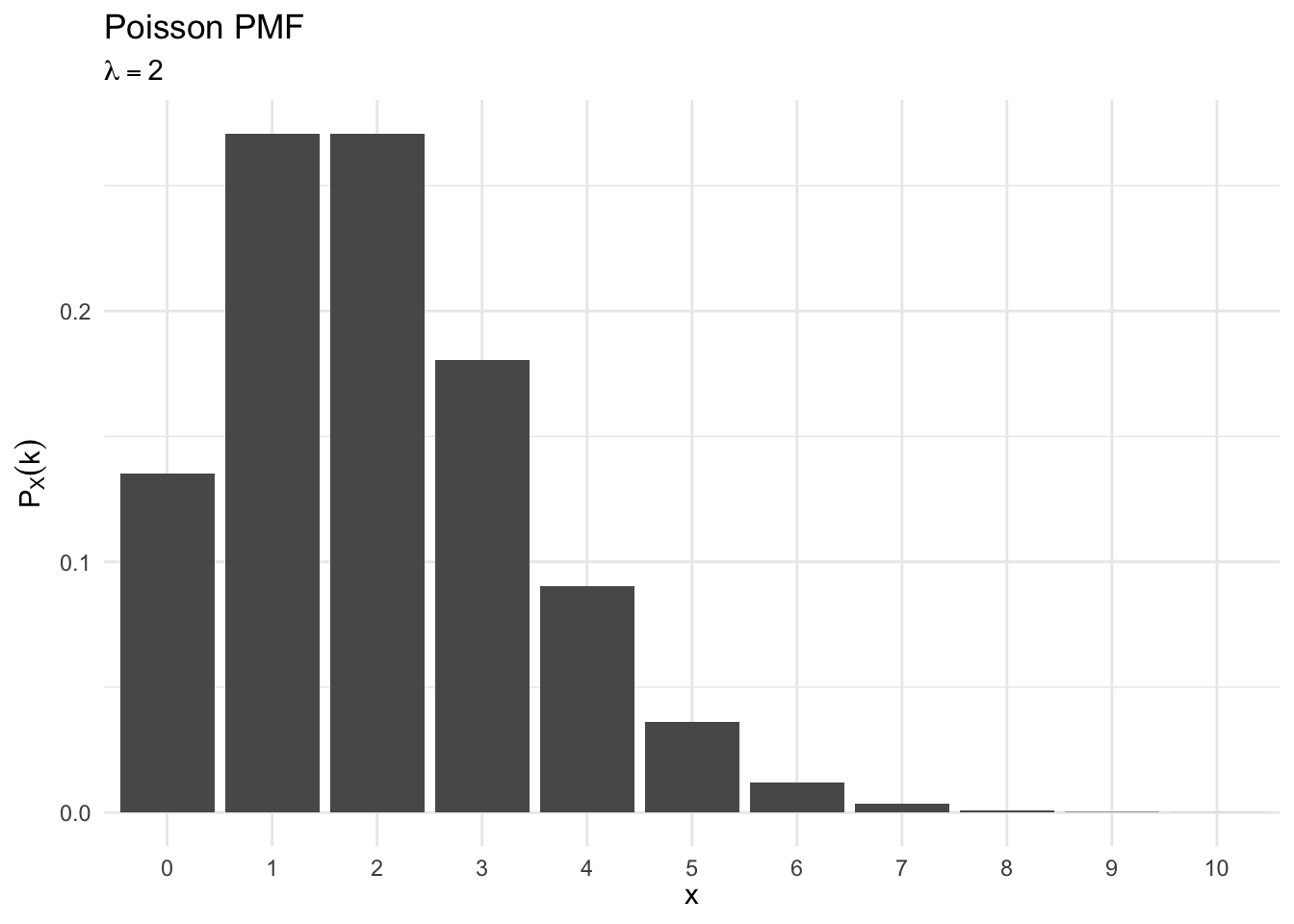

poisson_plot(5.5)

poisson_plot(78, max_n = 150)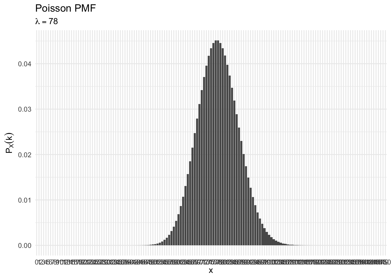

Example

Suppose the number of threats a president makes in a term is given by \(X \sim \text{Poisson}(5)\)
What is the probability the president will make ten threats?

\[ \begin{eqnarray} P(X = 10) & = & e^{-\lambda} \frac{5^{10}}{10!} \end{eqnarray} \]

data_frame(n = 1:50,
           prob = dpois(n, 5)) %>%
  ggplot(aes(n, prob)) +
  geom_col() +
  labs(x = "Number of threats",
       y = "Probability")

Approximating a binomial random variable

The Poisson PMF with parameter \(\lambda\) is a good approximation for a binomial PMF with parameters \(n\) and \(p\)

\[e^{-\lambda} \frac{\lambda^{k}}{k!} \approx {{N}\choose{k}}\pi^{k} (1- \pi)^{n-k}, \quad \text{if } k \ll n\]
- Provided \(\lambda = np\), \(n\) is very large, and \(p\) is very small
Sometimes using the Poisson PMF results in simpler models and easier calculations
Example
- \(n = 100\) and \(p = 0.01\)
- Using the binomial PMF
  
  \[\frac{100!}{95! 5!} \times 0.01^5 (1 - 0.01)^{95} = 0.00290\]
- Using the Poisson PMF with \(\lambda = np = 100 \times 0.01 = 1\)
  
  \[e^{-1} \frac{1}{5!} = 0.00306\]

Functions of random variables

Given a random variable \(X\), you may wish to create a new random variable \(Y\) using transformations of \(X\)
This could be a linear function of the form

\[Y = g(X) = aX + b\]
where \(a\) and \(b\) are scalars
It could be a logarithmic transformation \(g(X) = \log(X)\)
If \(Y = g(X)\) is a function of a random variable \(X\), then \(Y\) is also a random variable
All outcomes in the sample space defined with a numerical value \(x\) for \(X\) also have a numerical value \(y = g(x)\) for \(Y\)

Expectation, mean, and variance

PMF of a random variable \(X\) provides several numbers, the probabilities of all possible values of \(X\)
Often desirable to summarize this information into a single representative number
Expectation of \(X\) - weighted average of the possible values of \(X\)

Motivation

Consider spinning a wheel of fortune many times. At each spin, one of the numbers \(m_1, m_2, \ldots, m_n\) comes up with corresponding probability \(p_1, p_2, \ldots, p_n\), and this is your monetary reward from that spin. What is the amount of money that you “expect” to get “per spin”? The terms “expect” and “per spin” are a little ambiguous, but here is a reasonable interpretation.

Suppose you spin the wheel \(k\) times, and that \(k_i\) is the number of times that the outcome is \(m_i\). Then, the total amount received is \(m_1 k_1 + m_2 k_2 + \ldots + m_n k_n\). The amount received per spin is a simple average:

\[M = \frac{m_1 k_1 + m_2 k_2 + \ldots + m_n k_n}{k}\]

If the number of spins \(k\) is very large and we interpret probabilities as relative frequencies, we could anticipate that \(m_i\) comes up a fraction of times roughly equal to \(p_i\):

\[\frac{k_i}{k} \approx p_i, i = 1, \ldots,n\]

Thus, the amount of money you “expect” to receive is

\[M = \frac{m_1 k_1 + m_2 k_2 + \ldots + m_n k_n}{k} \approx m_1p_1 + m_2p_2 + \ldots + m_np_n\]

Expectation

Define expected value (known as expectation or the mean) of a random variable \(X\), with PMF \(p_X\) as

\[ \begin{eqnarray} \E[X] & = & \sum_{x:p(x)>0} x p(x) \end{eqnarray} \]

where \(\sum_{x:p(x)>0}\) is all values of \(X\) with probability greater than 0
In words: for all values of \(x\) with \(p(x)\) greater than zero, take the weighted average of the values

Example of expected value

Suppose \(X\) is number of units assigned to treatment, in one of our previous example.

\[ \begin{equation} X = \left \{ \begin{array} {ll} 0 \text{ if } (C, C, C) \\ 1 \text{ if } (T, C, C) \text{ or } (C, T, C) \text{ or } (C, C, T) \\ 2 \text{ if } (T, T, C) \text{ or } (T, C, T) \text{ or } (C, T, T) \\ 3 \text{ if } (T, T, T) \end{array} \right. \end{equation} \]
What is \(E[X]\)?

\[ \begin{eqnarray} \E[X] & = & 0\times \frac{1}{8} + 1 \times \frac{3}{8} + 2 \times \frac{3}{8} + 3 \times \frac{1}{8} \\ & = & 1.5 \end{eqnarray} \]
Essentially a weighted average, or the average outcome (value in the middle of the range)
Gives us a measure of central tendency

Variance, moments, and the expected value rule

Other quantities we care about include variance and moments

Moments

1st moment: \(\E[X^1] = \E[X]\) - that is, the mean
2nd moment: \(\E[X^2]\)
\(n\)th moment: \(\E[X^n]\)

Variance

\(\Var(X)\)
Defined as the expected value of the random variable \((X - \E[X])^2\)

\[ \begin{align} \Var(X) &= \E[(X - \E[X])^2] \end{align} \]
- Since \((X - \E[X])^2\) can only take non-negative values, variance is always non-negative
Measure of dispersion of \(X\) around its mean
We will define the standard deviation of \(X\), \(\sigma_X = \sqrt{\Var(X)}\)
- Standard deviation is easier to interpret sometimes since it is in the same units as \(X\)

Calculating variance of a random variable

We could generate the PMF of the random variable \((X - \E[X])^2\), then calculate the expectation of this function
- It is just a linear function
Instead, we can take a shortcut
Expected value rule for functions of random variables - let \(X\) be a random variable with PMF \(p_X\), and let \(g(X)\) be a function of \(X\). Then, the expected value of the random variable \(g(X)\) is given by
\[\E[g(X)] = \sum_{x} g(x) p_X(x)\]
This allows us to rewrite our variance formula:

\[ \begin{align} \Var(X) &= \E[(X - \E[X])^2] \\ \Var(X) &= \E[X^2] - \E[X]^2 \end{align} \]
- Just need the first and second moments to calculate variance

Practice calculating expectation and variance

Bernoulli variable

Suppose \(Y \sim \text{Bernoulli}(\pi)\)

\[ \begin{eqnarray} E[Y] & = & 1 \times P(Y = 1) + 0 \times P(Y = 0) \nonumber \\ & = & \pi + 0 (1 - \pi) \nonumber = \pi \\ \text{var}(Y) & = & E[Y^2] - E[Y]^2 \nonumber \\ E[Y^2] & = & 1^{2} P(Y = 1) + 0^{2} P(Y = 0) \nonumber \\ & = & \pi \nonumber \\ \text{var}(Y) & = & \pi - \pi^{2} \nonumber \\ & = & \pi(1 - \pi ) \nonumber \end{eqnarray} \]
\(E[Y] = \pi\)
Var\((Y) = \pi(1- \pi)\)
What is the maximum variance?

\[ \begin{eqnarray} \text{var}(Y) & = & \pi - \pi^{2} \nonumber \\ & = & 0.5(1 - 0.5 ) \\ & = & 0.25 \end{eqnarray} \]

Binomial

\[Z = \sum_{i=1}^{N} Y_{i} \text{ where } Y_{i} \sim \text{Bernoulli}(\pi)\]

\[ \begin{eqnarray} E[Z] & = & E[Y_{1} + Y_{2} + Y_{3} + \ldots + Y_{N} ] \\ & = & \sum_{i=1}^{N} E[Y_{i} ] \\ & = & N \pi \\ \text{var}(Z) & = & \sum_{i=1}^{N} \text{var}(Y_{i}) \\ & = & N \pi (1-\pi) \end{eqnarray} \]

Decision making using expected values

Optimizes the choice between several candidate decisions that result in random rewards
View the expected reward of a decision as its average payoff over a large number of trials
Choose a decision with maximum expected reward

Example: going to war

Suppose country \(1\) is engaged in a conflict and can either win or lose.
Define \(Y = 1\) if the country wins and \(Y = 0\) otherwise.
Then,

\[ \begin{eqnarray} Y &\sim & \text{Bernoulli}(\pi) \end{eqnarray} \]
Suppose country \(1\) is deciding whether to fight a war.
Engaging in the war will cost the country \(c\).
If they win, country \(1\) receives \(B\).
What is \(1\)’s expected utility from fighting a war?

\[ \begin{eqnarray} E[U(\text{war})] & = & (\text{Utility}|\text{win})\times P(\text{win}) + (\text{Utility}| \text{lose})\times P(\text{lose}) \\ &= & (B - c) P(Y = 1) + (- c) P(Y = 0 ) \\ & = & B \times p(Y = 1) - c(P(Y = 1) + P(Y = 0)) \\ & = & B \times \pi - c \end{eqnarray} \]
Based on your beliefs about the appropriate values for \(B, \pi, c\), you can decide whether to engage in the war
- If expected utility is greater than 0, you should decide to go to war
- If expected utility is less than 0, you should decide not to go to war

Cumulative distribution function

The cumulative distribution function (CDF) defines the the cumulative probability \(F_X(x)\) up to the value of \(x\). For a discrete random variable \(X\), we define the CDF \(F_X\) which provides the probability \(\Pr (X \leq x)\). For every \(x\)

\[F_X(x) = \Pr (X \leq x) = \sum_{k \leq x} p_X(k)\]

Any random variable associated with a given probability model has a CDF. Basic properties of CDFs for discrete random variables are:

\(F_X\) is monotonically nodecreasing – if \(x \leq y\), then \(F_X(x) \leq F_X(y)\)
\(F_X(x)\) tends to \(0\) as \(x \rightarrow -\infty\), and to \(1\) as \(x \rightarrow \infty\)
\(F_X(x)\) is a piecewise constant function of \(x\)
If \(X\) is discrete and takes integer values, the PMF and the CDF can be obtained from each other by summing or differencing:

\[F_X(k) = \sum_{i = -\infty}^k p_X(i),\] \[p_X(k) = \Pr (X \leq k) - \Pr (X \leq k-1) = F_X(k) - F_X(k-1)\]

for all integers \(k\)

Common CDFs

bernouli_cdf_plot <- function(p){
  df <- data_frame(x = 0:1,
                   pmf = dbinom(x = x, size = 1, prob = p),
                   cdf = pbinom(q = x, size = 1, prob = p)) %>%
    mutate(x = factor(x))
  
  ggplot(df, aes(x, pmf)) +
    geom_col() +
    labs(title = "Bernouli PMF",
         subtitle = bquote(pi == .(p)),
         x = expression(x),
         y = expression(P[X] (k))) +
    ggplot(df, aes(x, cdf)) +
    geom_col() +
    labs(title = "Bernouli CDF",
         subtitle = bquote(pi == .(p)),
         x = expression(x),
         y = expression(F[X] (k)))
}

bernouli_cdf_plot(.5)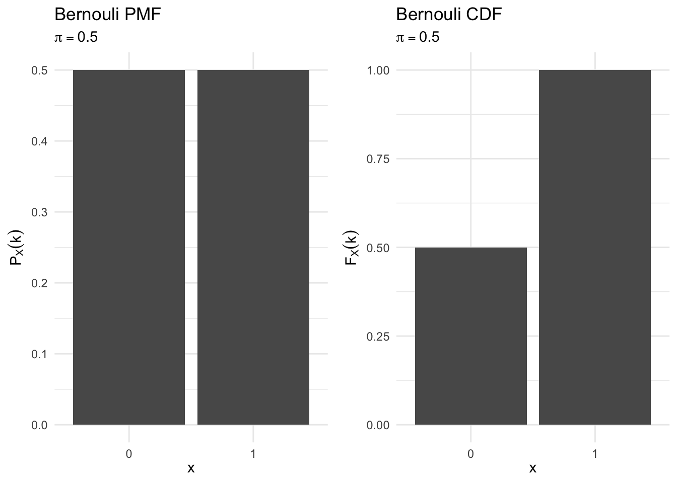

bernouli_cdf_plot(.7)

bernouli_cdf_plot(.3)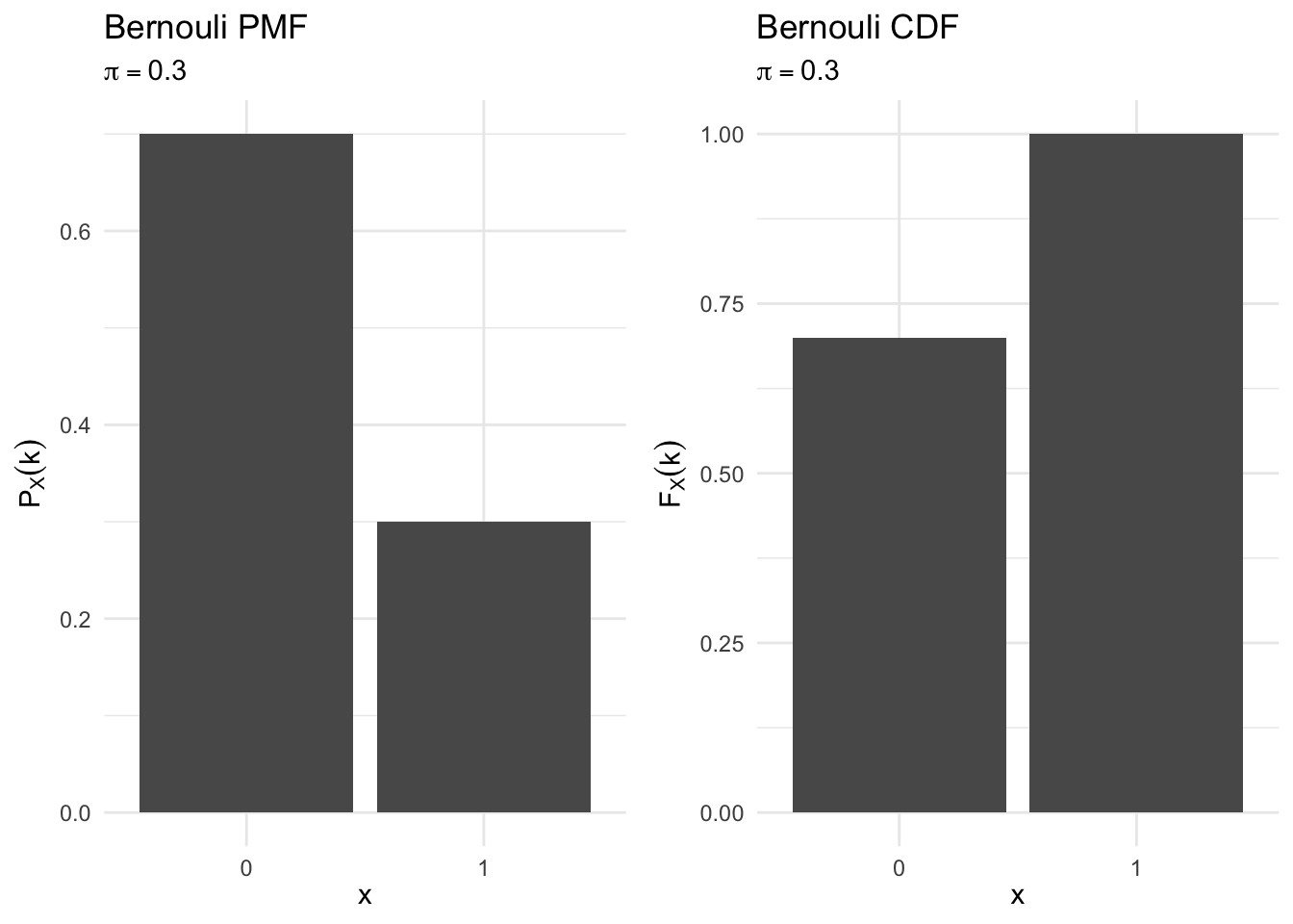

binomial_cdf_plot <- function(n, p){
  df <- data_frame(x = 0:n,
                   pmf = dbinom(x = x, size = n, prob = p),
                   cdf = pbinom(q = x, size = n, prob = p))
  
  ggplot(df, aes(x, pmf)) +
    geom_col() +
    labs(title = "Binomial PMF",
         subtitle = bquote(n == .(n) ~ p == .(p)),
         x = expression(x),
         y = expression(P[X] (k))) +
    ggplot(df, aes(x, cdf)) +
    geom_col() +
    labs(title = "Binomial CDF",
         subtitle = bquote(n == .(n) ~ p == .(p)),
         x = expression(x),
         y = expression(F[X] (k)))
}

binomial_cdf_plot(10, .5)

binomial_cdf_plot(10, .3)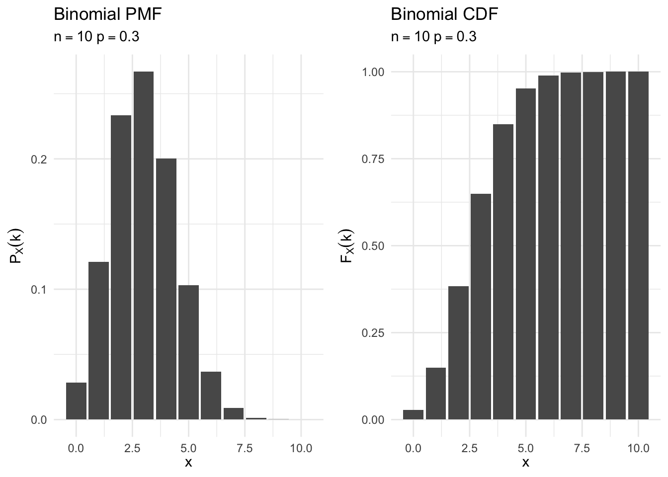

binomial_cdf_plot(100, .2)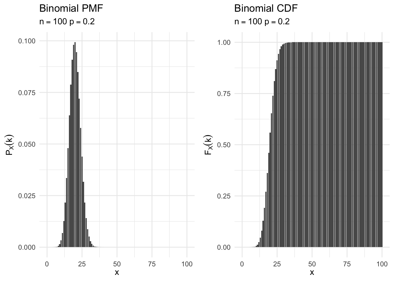

binomial_cdf_plot(100, .8)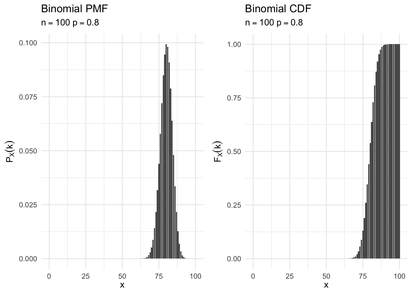

geometric_cdf_plot <- function(p){
  df <- data_frame(x = 0:20,
                   pmf = dgeom(x = x, prob = p),
                   cdf = pgeom(q = x, prob = p)) %>%
    mutate(x = x + 1)
  
  ggplot(df, aes(x, pmf)) +
    geom_col() +
    labs(title = "Geometric PMF",
         subtitle = bquote(p == .(p)),
         x = expression(x),
         y = expression(P[X] (k))) +
    ggplot(df, aes(x, cdf)) +
    geom_col() +
    labs(title = "Geometric CDF",
         subtitle = bquote(p == .(p)),
         x = expression(x),
         y = expression(F[X] (k)))
}

geometric_cdf_plot(.5)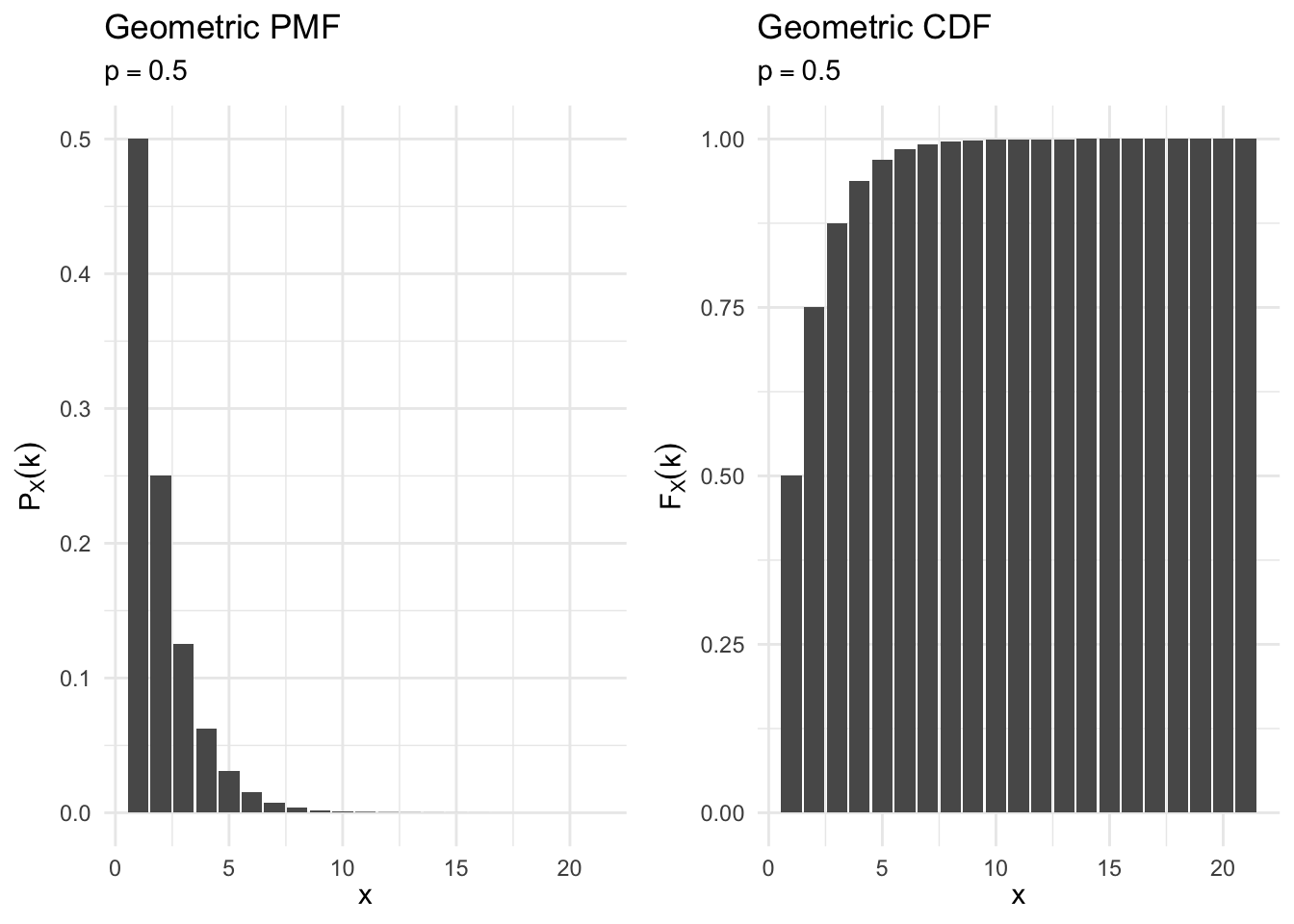

geometric_cdf_plot(.7)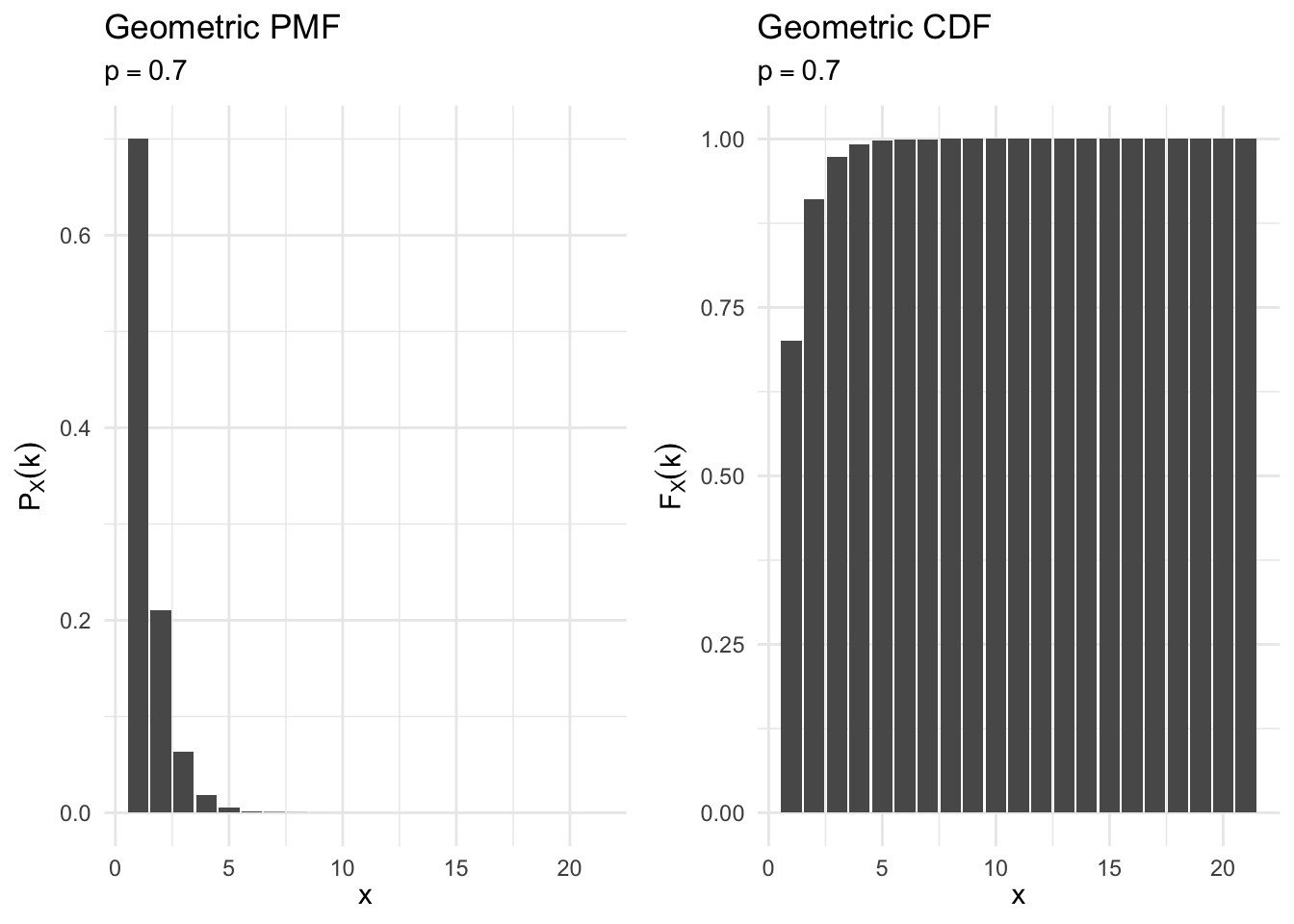

geometric_cdf_plot(.2)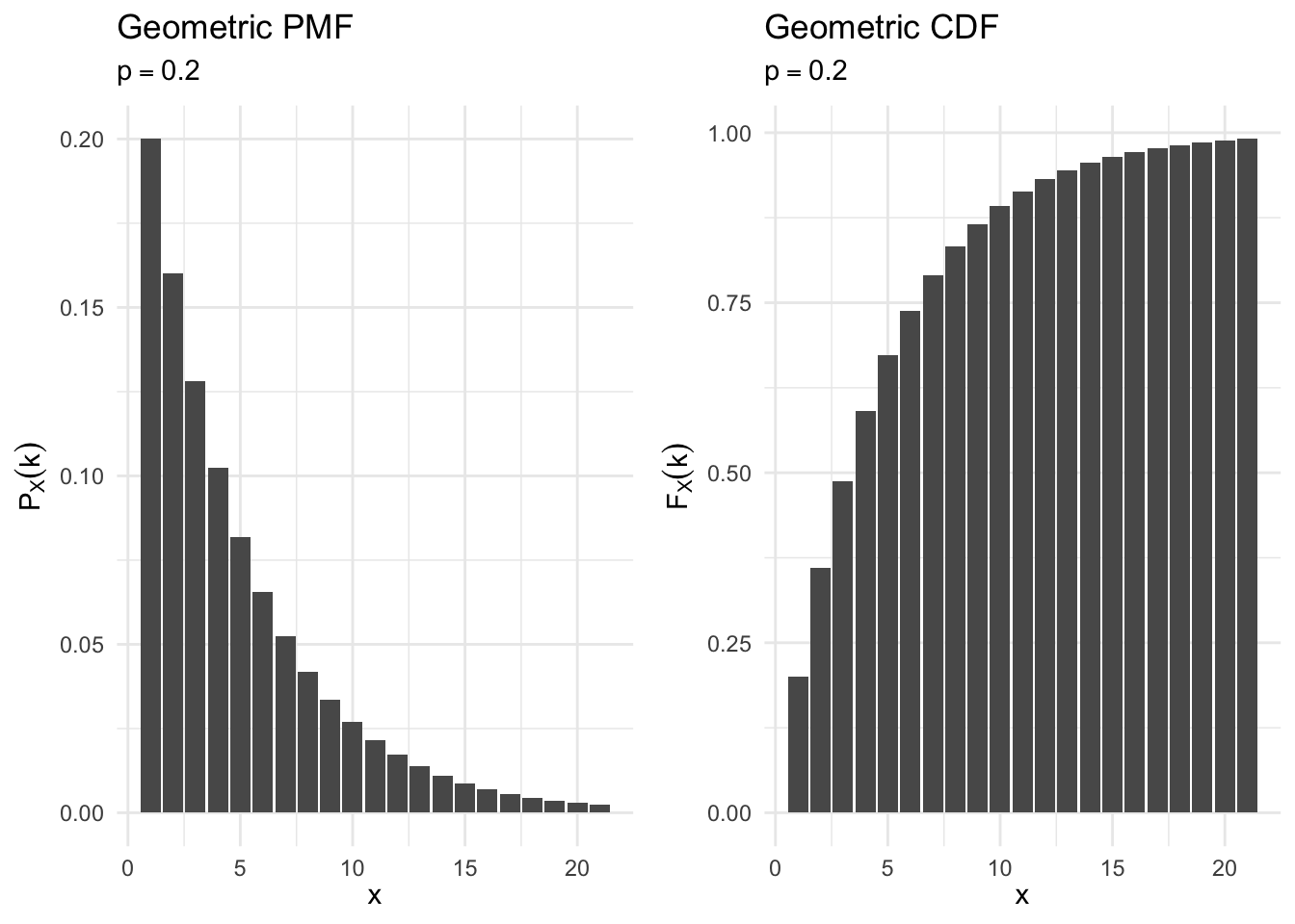

poisson_cdf_plot <- function(lambda, max_n = 10){
  df <- data_frame(x = 0:max_n,
                   pmf = dpois(x = x, lambda = lambda),
                   cdf = ppois(q = x, lambda = lambda))
  
  ggplot(df, aes(x, pmf)) +
    geom_col() +
    labs(title = "Poisson PMF",
         subtitle = bquote(lambda == .(lambda)),
         x = expression(x),
         y = expression(P[X] (k))) +
    ggplot(df, aes(x, cdf)) +
    geom_col() +
    labs(title = "Poisson CDF",
         subtitle = bquote(lambda == .(lambda)),
         x = expression(x),
         y = expression(F[X] (k)))
}

poisson_cdf_plot(2)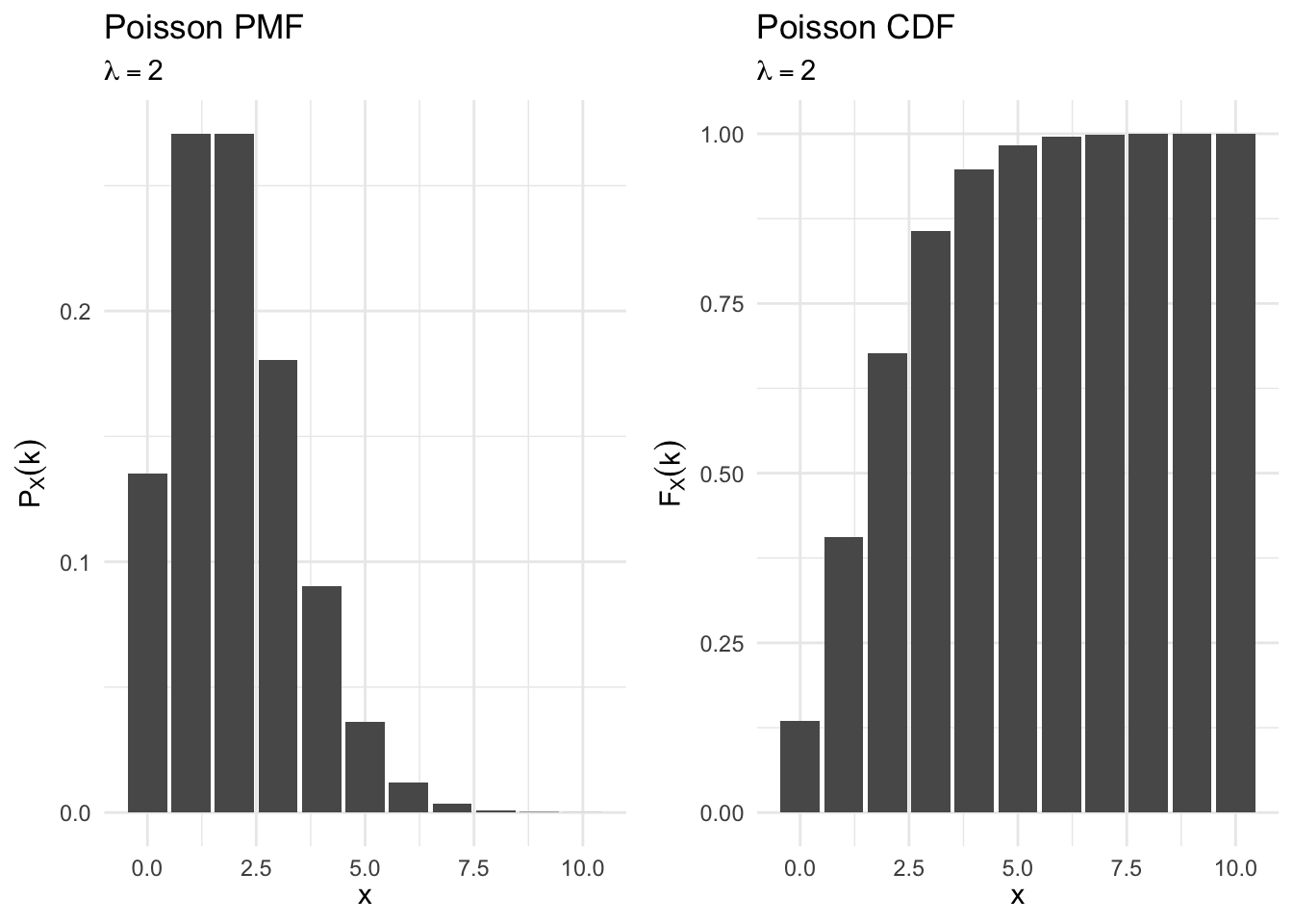

poisson_cdf_plot(5.5)

poisson_cdf_plot(78, max_n = 150)

Functions for working with probabilities

Most common probability distributions have a core set of functions in R that you can use to calculate probabilities, cumulative probabilities, and generate simulated random variables. They follow a common naming scheme:

d*() - density function, calculates exact probability for a given \(x\)
p*() - distribution function, calculates cumulative probability for a given \(\Pr(X \leq x)\)
r*() - random data generation, generates \(n\) values from a specified probability distribution with known parameters

Binomial

To find this binomial probability	Use this R command
\(\Pr(x = a)\)	`dbinom(x = a, size = n, prob = p)`
\(\Pr(x \leq a)\)	`pbinom(q = a, size = n, prob = p)`
\(\Pr(x < a)\)	`pbinom(q = a - 1, size = n, prob = p)`
\(\Pr(x \geq a) = 1 - \Pr(x \leq a) = 1 - \Pr (x \leq a-1)\)	`1 - pbinom(q = a - 1, size = n, prob = p)`
\(\Pr(x > a) = 1 - \Pr(x \leq a)\)	`1 - pbinom(q = a, size = n, prob = p)`

Calculating probabilities

\[ \begin{eqnarray} p_X(k) & = & {{N}\choose{k}}\pi^{k} (1- \pi)^{n-k} \end{eqnarray} \]

\(N = 10, k = 5, \pi = .5\)

N <- 10
k <- 5
prob <- .5

To find this binomial probability	Use this R command	Result
\(\Pr(x = 5)\)	`dbinom(x = k, size = N, prob = prob)`	0.246
\(\Pr(x \leq 5)\)	`pbinom(q = k, size = N, prob = prob)`	0.623
\(\Pr(x < 5)\)	`pbinom(q = k - 1, size = N, prob = prob)`	0.377
\(\Pr(x \geq 5) = 1 - \Pr(x \leq 5) = 1 - \Pr (x \leq 5-1)\)	`1 - pbinom(q = k - 1, size = N, prob = prob)`	0.623
\(\Pr(x > 5) = 1 - \Pr(x \leq 5)\)	`1 - pbinom(q = k - 1, size = N, prob = prob)`	0.623

\(N = 20, k = 5, \pi = .4\)

N <- 20
k <- 5
prob <- .4

To find this binomial probability	Use this R command	Result
\(\Pr(x = 5)\)	`dbinom(x = k, size = N, prob = prob)`	0.075
\(\Pr(x \leq 5)\)	`pbinom(q = k, size = N, prob = prob)`	0.126
\(\Pr(x < 5)\)	`pbinom(q = k - 1, size = N, prob = prob)`	0.051
\(\Pr(x \geq 5) = 1 - \Pr(x \leq 5) = 1 - \Pr (x \leq 5-1)\)	`1 - pbinom(q = k - 1, size = N, prob = prob)`	0.949
\(\Pr(x > 5) = 1 - \Pr(x \leq 5)\)	`1 - pbinom(q = k - 1, size = N, prob = prob)`	0.949

\(N = 1, k = 1, \pi = .4\) (i.e. a Bernoulli random variable)

N <- 1
k <- 1
prob <- .4

To find this Bernoulli probability	Use this R command	Result
\(\Pr(x = 1)\)	`dbinom(x = k, size = N, prob = prob)`	0.4
\(\Pr(x \leq 1)\)	`pbinom(q = k, size = N, prob = prob)`	1
\(\Pr(x < 1)\)	`pbinom(q = k - 1, size = N, prob = prob)`	0.6
\(\Pr(x \geq 1) = 1 - \Pr(x \leq 1) = 1 - \Pr (x \leq 1-1)\)	`1 - pbinom(q = k - 1, size = N, prob = prob)`	0.4
\(\Pr(x > 1) = 1 - \Pr(x \leq 1)\)	`1 - pbinom(q = k - 1, size = N, prob = prob)`	0.4

Simulating random variables

\(N = 10, \pi = .5\)
Simulate 1000 observations

set.seed(1234)

# store in a vector
rbinom(1000, size = 10, prob = .5)

##    [1]  3  5  5  6  7  6  1  4  6  5  6  5  4  7  4  7  4  4  4  4  4  4  3
##   [24]  2  4  6  5  7  7  2  5  4  4  5  4  6  4  4  9  6  5  6  4  5  4  5
##   [47]  6  5  4  6  3  4  6  5  3  5  5  6  4  7  7  2  4  2  4  6  4  5  2
##   [70]  5  3  7  2  6  3  5  5  3  4  6  7  5  3  5  4  7  5  4  3  7  3  7
##   [93]  3  3  3  5  4  2  4  6  2  5  4  4  3  4  3  3  5  2  6  3  8  3  4
##  [116]  7  8  4  3  6  6  7  9  7  5  4  4  5  5  4  8  6  3  5  7  5  7  5
##  [139]  6  7  5  8  4  5  4  6  6  5  8  5  5  4  3  7  4  8  5  9  4  5  5
##  [162]  5  5  4  3  6  5  3  6  4  6  5  6  5  4  6  5  5  3  4  5  4  5  3
##  [185]  8  2  7  6  4  6  6  9  3  7  6  6  7  6  8  6  6  5  4  6  5  6  4
##  [208]  5  4  8  5  4  4  6  5  7  6  6  5  7  5  2  4  4  3  5  6  4  5  5
##  [231]  6  5  3  6  5  4  6  4  5  9  5  4  4  6  8  5  6  5  8  6  5  5  4
##  [254]  4  3  5  4  1  5  5  7  2  5  4  3  3  6  2  2  6  4  6  4  6  2  5
##  [277]  6  5  4  4  4  5  7  6  6  4  5  4  6  6  6  5  8  4  5  6  6  3  6
##  [300]  4  4  8  5  5  8  5  4  9  5  6  7  6  5  5  3  4  4  5  4  7  4  7
##  [323]  5  3  4  4  5  4  6  7  6  7  8  4  5  5  4  2  7  5  8  4  5  8  4
##  [346]  4  2  6  7  2  4  6  3  6  9  7  5  6  5  6  1  5  5  4  7  8  6  4
##  [369]  6  6  8  4  7  5  4  5  6  3  5  6  4  4  1  3  4  3  6  4  8  8  6
##  [392]  6  6  6  3  7  5  5  2  4  6  5  6  6  5  4  6  3  5  5  6  6  8  4
##  [415]  7  5  5  6  3  5  6  7  4  3  7  4  2  5  4  4  6  6  5  7  4  6  5
##  [438]  7  6  5  6  7  6  5  8  5  7  6  5  2  4  6  9  8  6  6  4  5  5  2
##  [461]  4  7  5  5  4  4  5  5  6  5  3  4  0  8  5  8  5  5  6  3  5  5  6
##  [484]  4  3  3  6  6  6  3  5  6  7  4  6  4  5  3  5  5  6  6  7  2  6  7
##  [507]  6  7  3  6  4  8  7  5  3  6  5  3  6  4  7  4  4  7  5  6  2  2  6
##  [530]  4  4  6  5  6  3  9  6  6  6  5  5  5  8  4  6  5  7  7  8  7  4  4
##  [553]  6  3  7  8  5  2  6  7  3  9  6  7  4  7  6  5  4  3  6  6  4  6  5
##  [576]  5  3  5  5  6  7  2  5  4  2  4  4  8  8  5  8  7  3  5  4  6  6  6
##  [599]  6  3  4  4  3  5  5  5  7  4  5  5  4  6  4  3  8  5  4  6  6  5  7
##  [622]  2  6  6  4  7  5  8  4  5  7  5  5  5  7  7  4  7  4  4  5  4  5  7
##  [645]  4  4  3  7  5  6  4  6  7  5  3  5  7  2  4  7  5  8  6  2  4  5  6
##  [668]  4  5  6  3  7  5  4  8  7  5  7  4  8  5  3  6  4  7  4  7  2  5  5
##  [691]  7  5  4  5  1  3  4  5  4  6  1  5  6  5  4  3  5  6  3  5  6  8  8
##  [714]  3  4  4  5  4  8  3  6  3  8  1  5  8  5  4  4  8  7  2  3  5  5  6
##  [737]  5  6  8  7  4  3  3  4  5  0  5  6  4  6  5  6  5  7  4  7  6  7  4
##  [760]  5  2  6  1  5  4  5  7  5  6  4  7  7  7  3  6  5  3  4  5  4  7  3
##  [783]  0  4  4  6  7  2  6  3  6  3  6  5  6  4  5  6  4  7  3  7  5  4  4
##  [806]  5  4  5  6  5  5  4  7  6  3  4  4  6  5  5  3  4  5  5  4  6  2  5
##  [829]  5  5  4  6  7  7  4  6  6  4  5  6  3  5  6  4  5  7  5  7  6  6  5
##  [852]  8  7  4  5  6  3  2  6  8  3  5  2  5  4  7  4  8  4  5  8  7  8  4
##  [875]  6  4  3  3  5  5  6  4  5  5  5  7  4  2  3  2  7  6  5  5  4  4  6
##  [898]  6  8  7  6  5  7  5  7  2  4  4  6  4  4  5  3  4  3  3  5  8  8  6
##  [921]  5  5  4  4  5  4  6  5  3  3  3  9  2  5  3  5  4  5  5  5  7  5  6
##  [944]  6  5  5  4  3  5  4  6  8  4  6  7  2  7  5  3  6  4  5  7  6  2  3
##  [967]  6  4  5  4 10  6  1  6  4  6  6  4  8  5  6  7  3  6  8  4  2  8  3
##  [990]  4  5  6  8  3  6  1  6  4  8  4

# store in a data frame
data_frame(x = rbinom(1000, size = 10, prob = .5))

## # A tibble: 1,000 x 1
##        x
##    <int>
##  1     7
##  2     5
##  3     3
##  4     4
##  5     6
##  6     5
##  7     5
##  8     3
##  9     8
## 10     8
## # ... with 990 more rows

Each simulation is a new draw from the same underlying probability distribution. The individual draws will not be identical:

rerun(.n = 10, rbinom(10, size = 10, prob = .5)) %>%
  bind_cols()

## # A tibble: 10 x 10
##       V1    V2    V3    V4    V5    V6    V7    V8    V9   V10
##    <int> <int> <int> <int> <int> <int> <int> <int> <int> <int>
##  1     3     2     7     5     5     4     7     4     5     7
##  2     4     7     7     5     5     5     5     3     2     6
##  3     5     6     7     4     4     7     3     7     3     6
##  4     5     4     2     5     8     5     4     4     5     3
##  5     3     5     3     1     5     6     3     5     4     5
##  6     6     4     7     5     8     7     8     6     5     4
##  7     6     4     4     5     4     5     4     4     6     2
##  8     2     6     4     4     4     5     4     6     1     7
##  9     6     6     5     3     4     3     3     6     8     4
## 10     4     4     3     5     5     5     2     4     4     5

But (given a large enough sample size), they will be from the same underlying distribution:

rerun(.n = 9, rbinom(1000, size = 10, prob = .5)) %>%
  bind_cols() %>%
  gather(var, value) %>%
  ggplot(aes(value)) +
  geom_bar() +
  facet_wrap(~var) +
    labs(title = "Simulated draws from a Binomial PMF",
         subtitle = expression(n == 10 ~ pi == .5),
         x = expression(x),
         y = expression(p[X] (k)))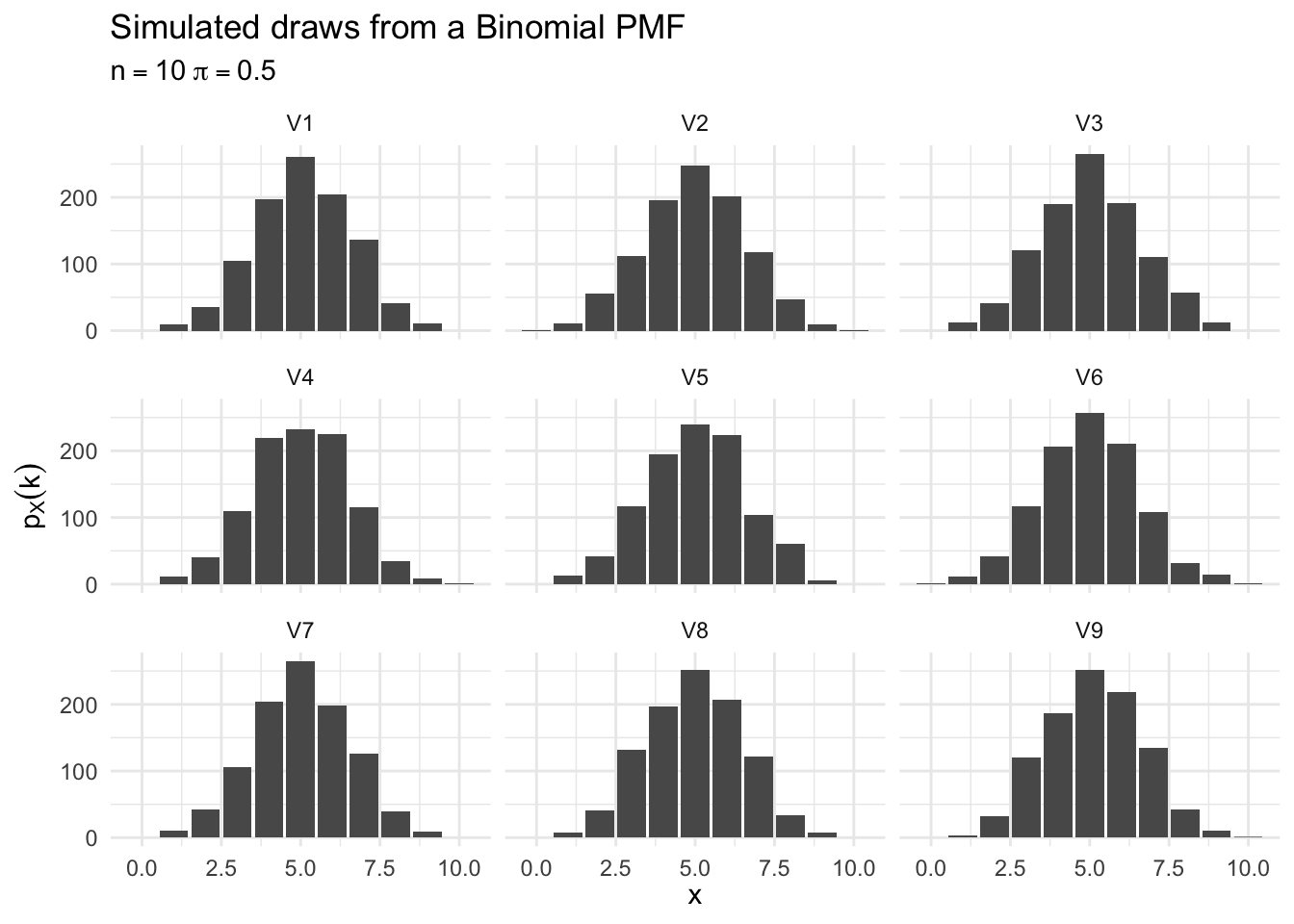

Setting the seed (set.seed()) of your random number generator ensures consistent output from any r*() function. For example:

# draw #1
set.seed(1234)
rbinom(10, size = 10, prob = .5)

##  [1] 3 5 5 6 7 6 1 4 6 5

# draw #2
set.seed(1234)
rbinom(10, size = 10, prob = .5)

##  [1] 3 5 5 6 7 6 1 4 6 5

Poisson

To find this Poisson probability	Use this R command
\(\Pr(x = a)\)	`dpois(x = a, lambda = p)`
\(\Pr(x \leq a)\)	`ppois(q = a, lambda = p)`
\(\Pr(x < a)\)	`ppois(q = a - 1, lambda = p)`
\(\Pr(x \geq a) = 1 - \Pr(x \leq a) = 1 - \Pr (x \leq a-1)\)	`1 - ppois(q = a - 1, lambda = p)`
\(\Pr(x > a) = 1 - \Pr(x \leq a)\)	`1 - ppois(q = a, lambda = p)`

Examples

\(N = 3, \lambda = 5\)

N <- 3
lambda <- 5

To find this Poisson probability	Use this R command	Results
\(\Pr(x = 3)\)	`dpois(x = N, lambda = lambda)`	0.14
\(\Pr(x \leq 3)\)	`ppois(q = N, lambda = lambda)`	0.265
\(\Pr(x < 3)\)	`ppois(q = N - 1, lambda = lambda)`	0.125
\(\Pr(x \geq 3) = 1 - \Pr(x \leq 3) = 1 - \Pr (x \leq 3-1)\)	`1 - ppois(q = N - 1, lambda = lambda)`	0.875
\(\Pr(x > 3) = 1 - \Pr(x \leq 3)\)	`1 - ppois(q = N, lambda = lambda)`	0.735

\(N = 12, \lambda = 17.3\)

N <- 12
lambda <- 17.3

To find this Poisson probability	Use this R command	Results
\(\Pr(x = 3)\)	`dpois(x = N, lambda = lambda)`	0.046
\(\Pr(x \leq 3)\)	`ppois(q = N, lambda = lambda)`	0.121
\(\Pr(x < 3)\)	`ppois(q = N - 1, lambda = lambda)`	0.075
\(\Pr(x \geq 3) = 1 - \Pr(x \leq 3) = 1 - \Pr (x \leq 3-1)\)	`1 - ppois(q = N - 1, lambda = lambda)`	0.925
\(\Pr(x > 3) = 1 - \Pr(x \leq 3)\)	`1 - ppois(q = N, lambda = lambda)`	0.879

Simulating random variables

\(N = 12, \lambda = 17.3\)
Simulate 1000 observations

set.seed(1234)

# store in a vector
(X <- rpois(1000, lambda = 17.3))

##    [1] 12 18 18 14 19 14 21 14 15 10 17 21 16 15 20 14 17 15 17 17 20 15 13
##   [24] 20 21 31 24 11 23 12 22 15 13 12 15 20 17 13 13 25 20 27 17 14 15 12
##   [47] 16 18 21 26 17 18 17 18 14 14 29 17 18 14 16 20 20 19 15 17 15 18 24
##   [70] 21 15 27 22 21 19 18 17 20 19 16 26 14 17 18 17 16 14 17 15 20 12 13
##   [93] 17 16 14 17 18 20 18 14 14 17 29 15 17 17 15 23 19 16 19 18 24 18 19
##  [116] 18 15 16 16 27 20 19 16 13 15 21 13 16 18 19 24 17 15 16 14 15 19 10
##  [139] 12 23 19 20 17 15 19 21 25 22 15 11 15 12 19 26 19 19 13 17 15 20 18
##  [162] 20 18 20 24 21 17 12 22 12 10 14 16 14 23 18 22 17 17 18  9 29 20 14
##  [185] 10 16 13 16 18 14 16 17 19 17 19 12 19 13 22 18 18 18 19 21 19 20 12
##  [208] 24 18 20 11 21 15 20 10 14 20 27 18 17 18 14 21 25 14 13 17 18 13 21
##  [231] 21 18 10 13 16 16 21 27 24 24 12 19 19 12 13 16 13 14 11 15 17 10 15
##  [254] 23 18 18 17 21 21 15 17 15 22 20 19 16 17  9 18 21 15 14 12 14 16 13
##  [277] 12 21 22 17 22 14 11 15 18 16 12 10 25 12 16 25 21 25 17 16 15  7 18
##  [300] 17 26 14 28 20 21 22 23 18 18 18 18 18 15 21 18 11 15 26 22 19 19 17
##  [323] 13 22 14 13 16 13 12 20 16 15 14 16 16 20 23 19 13 12 13 17 20 17 23
##  [346] 17 12 24 16 16 23 26 17 22 15 12 18 14 18 13  8 18 15 18 21 16 16 22
##  [369] 14 14 16 24 17 13 14 11 27 18 17 17 18 18 20 17 12 19 15 10 12 16 20
##  [392] 11 18 30 26 14 20 11 14 12 18 22 24 21 12 16 12 16 10 15 17 12 25 15
##  [415] 15 20 23 14 22 23 16 22 17 14 22 14 17 18 18 20 16 24 19 12 14 15 16
##  [438] 28 15 17 14 12 18 19 19 11  9 14 16 15  5 15 14 21 16 11 23 13 13 13
##  [461] 18 21 16 14 14 11 15 12 19 18 16 19 14 14 16 15 15 19 21 17 15 18 15
##  [484] 13 15 10 21 20 13 23 12 13 17 19 17 11 13 18 13 25 13 15 24 13 16 17
##  [507] 22 16 22 17 18 18 18 18 19 19 21 21 17 12 22 23 19 18 21 12 19 16 18
##  [530] 21 16 16 19 12 19 16 26 13 15 18 15 19 18 16 19 12 14 19 24 22 27 18
##  [553] 18 21 23 24 14 13 20 21 19 23 16 12 25 13 26 15 16 17 20 13 17 24 25
##  [576] 15 14 19 16 12 22 21 22 15 14 23 16 17 18 20 16 27 13 20 12 17 17 20
##  [599] 16 17 22 17 14 19 19 14 12 14 14 16 20 18 21 28 12 14 18 16 11 18 28
##  [622] 19 23 21 17 15 22 15 19 24 16 18 20 12 13 15 19 22 16 12 16 17 17 14
##  [645] 21 12 13 23 13 16 15 24 23 14 14 13 21 26 18 14 12 17 15 14 11 19 19
##  [668] 14 16 19 10 18 13 17 15 14 15 17 13 16 20 18 17  9 20 15 16 18 10 18
##  [691] 20 19 14 15 15 21 24 21  9 17 17 21 20 16 16 11 20 17 17 23 20 31 11
##  [714] 21 19 17 16 15 18 14 15 14 25  9 15 15 14 18 14 17 12 11 26 23 23 20
##  [737] 15 19 12 19 17 18 20 13 12 13 18 23 21 17 20 16 21 22 12 16 18 16 24
##  [760]  9 27 16 23 20 24 27 18 13 16 21 20 18 17 19 21 22 14 19 18 17 21 16
##  [783] 18 13 17 18 26 19 20 15 13 10  9  9 13 14 15 23 12 15 17 15 16 15 17
##  [806] 13 25 15 15 16 21 18 18 17 14 14 25 14 14 12 16 22 17 10 16 23 21 18
##  [829] 19 17 17  9 17 13 16 20 17 19 15 15 19 18 18 19 16 13 22 18 17 13 16
##  [852] 14 20 18 14 17 19 33 18 23 17 19 16 26 22 16 16 17 17 14 20 11 20 20
##  [875] 14 14 16 13 16 23 21 18 19 25 17 17 23 19  7 13 17 16 20 13 18 19 23
##  [898] 18 20 22 15 20 18 24 17 29 18 16 17 29 13 13 17 13 18 17 20 24 21 14
##  [921] 18 19 17 14 15 17 26 24 12 17 16 16 21 12 17 13 19 12 19 25 12 22  7
##  [944] 14 14 14 17 13 18 13 16 14 22 18 11 27 20 10 23 20 14 17 19 13 17 22
##  [967] 17 23 13 23 19 22 21 14 13 17 13 21 17 14 21 20 25 22 19 26 19 16 15
##  [990] 16 18 11 10 19 15 17 28 14 21 23

What is the expected value of \(X\)? Its variance?

mean(X)

## [1] 17.4

var(X)

## [1] 17

Practice with probability distributions in R

Lincoln Tunnel

If 85% of vehicles arriving at the Lincoln Tunnel (connecting New Jersey and New York City) have either New York or New Jersey license plates, what is the probability that, of the next 20 vehicles, 2 or fewer (that is, 0, 1, or 2) will bear license plates from states other than New Jersey or New York?

Click for the solution

Set this up as a binomial distribution:

\[ \begin{eqnarray} p_X(k) & = & {{N}\choose{k}}\pi^{k} (1- \pi)^{n-k} \end{eqnarray} \]

where \(N = 20\) and \(p=0.15\). We need to calculate the probability that 0, 1, or 2 of the next cars will bear license plates from states other than New Jersey or New York. One way to state the problem is:

\[ \sum_{k = 0}^2 {{N}\choose{k}}\pi^{k} (1- \pi)^{n-k} = \sum_{k = 0}^2 {{20}\choose{k}} 0.15^{k} (1- 0.15)^{20-k} \]

In R, that is

dbinom(0, 20, 0.15) + dbinom(1, 20, 0.15) + dbinom(2, 20, 0.15)

## [1] 0.405

Alternatively, we can frame this in terms of the CDF and we want to know

\[F_X(x) = \Pr (X \leq 2) = \sum_{k \leq 2} p_X(k)\]

In R, we use the pbinom() function:

pbinom(2, 20, 0.15)

## [1] 0.405

Booking travel

Book4Less.com is an online travel website that offers competitive prices on airline and hotel bookings. During a typical weekday, the website averages 10 visits per minute.

What is the probability that there will be at least 7 but no more than 12 visits in the next minute?

Click for the solution

\[\sum_{k = 7}^{12} e^{-10} \frac{10^{k}}{k!}\]

\[F_X(x) = \Pr (7 \leq x \leq 12) = \sum_{k = 7}^{12} e^{-10} \frac{10^{k}}{k!}\]

dpois(7:12, 10)

## [1] 0.0901 0.1126 0.1251 0.1251 0.1137 0.0948

sum(dpois(7:12, 10))

## [1] 0.661

ppois(12, 10) - ppois(6, 10)

## [1] 0.661

What is the probability there will be more than 12 visits in the next minute?

Click for the solution

\[\sum_{k = 13}^{\infty} e^{-10} \frac{10^{k}}{k!}\]

\[F_X(x) = \Pr (x > 12) = \sum_{k = 13}^{\infty} e^{-10} \frac{10^{k}}{k!}\]

sum(dpois(13:50, 10))

## [1] 0.208

1 - ppois(12, 10)

## [1] 0.208

Acknowledgements

Material drawn from Introduction to Probability (2nd edition) by Bertsekas and Tsitsiklis

Session Info

devtools::session_info()

## Session info -------------------------------------------------------------

##  setting  value                       
##  version  R version 3.5.1 (2018-07-02)
##  system   x86_64, darwin15.6.0        
##  ui       X11                         
##  language (EN)                        
##  collate  en_US.UTF-8                 
##  tz       America/Chicago             
##  date     2018-10-25

## Packages -----------------------------------------------------------------

##  package    * version date       source                              
##  assertthat   0.2.0   2017-04-11 CRAN (R 3.5.0)                      
##  backports    1.1.2   2017-12-13 CRAN (R 3.5.0)                      
##  base       * 3.5.1   2018-07-05 local                               
##  bindr        0.1.1   2018-03-13 CRAN (R 3.5.0)                      
##  bindrcpp   * 0.2.2   2018-03-29 CRAN (R 3.5.0)                      
##  broom      * 0.5.0   2018-07-17 CRAN (R 3.5.0)                      
##  cellranger   1.1.0   2016-07-27 CRAN (R 3.5.0)                      
##  cli          1.0.0   2017-11-05 CRAN (R 3.5.0)                      
##  codetools    0.2-15  2016-10-05 CRAN (R 3.5.1)                      
##  colorspace   1.3-2   2016-12-14 CRAN (R 3.5.0)                      
##  compiler     3.5.1   2018-07-05 local                               
##  crayon       1.3.4   2017-09-16 CRAN (R 3.5.0)                      
##  datasets   * 3.5.1   2018-07-05 local                               
##  devtools     1.13.6  2018-06-27 CRAN (R 3.5.0)                      
##  digest       0.6.15  2018-01-28 CRAN (R 3.5.0)                      
##  dplyr      * 0.7.6   2018-06-29 cran (@0.7.6)                       
##  evaluate     0.11    2018-07-17 CRAN (R 3.5.0)                      
##  forcats    * 0.3.0   2018-02-19 CRAN (R 3.5.0)                      
##  ggplot2    * 3.0.0   2018-07-03 CRAN (R 3.5.0)                      
##  glue         1.3.0   2018-07-17 CRAN (R 3.5.0)                      
##  graphics   * 3.5.1   2018-07-05 local                               
##  grDevices  * 3.5.1   2018-07-05 local                               
##  grid         3.5.1   2018-07-05 local                               
##  gtable       0.2.0   2016-02-26 CRAN (R 3.5.0)                      
##  haven        1.1.2   2018-06-27 CRAN (R 3.5.0)                      
##  hms          0.4.2   2018-03-10 CRAN (R 3.5.0)                      
##  htmltools    0.3.6   2017-04-28 CRAN (R 3.5.0)                      
##  httr         1.3.1   2017-08-20 CRAN (R 3.5.0)                      
##  jsonlite     1.5     2017-06-01 CRAN (R 3.5.0)                      
##  knitr        1.20    2018-02-20 CRAN (R 3.5.0)                      
##  lattice      0.20-35 2017-03-25 CRAN (R 3.5.1)                      
##  lazyeval     0.2.1   2017-10-29 CRAN (R 3.5.0)                      
##  lubridate    1.7.4   2018-04-11 CRAN (R 3.5.0)                      
##  magrittr     1.5     2014-11-22 CRAN (R 3.5.0)                      
##  memoise      1.1.0   2017-04-21 CRAN (R 3.5.0)                      
##  methods    * 3.5.1   2018-07-05 local                               
##  modelr       0.1.2   2018-05-11 CRAN (R 3.5.0)                      
##  munsell      0.5.0   2018-06-12 CRAN (R 3.5.0)                      
##  nlme         3.1-137 2018-04-07 CRAN (R 3.5.1)                      
##  patchwork  * 0.0.1   2018-09-06 Github (thomasp85/patchwork@7fb35b1)
##  pillar       1.3.0   2018-07-14 CRAN (R 3.5.0)                      
##  pkgconfig    2.0.2   2018-08-16 CRAN (R 3.5.1)                      
##  plyr         1.8.4   2016-06-08 CRAN (R 3.5.0)                      
##  purrr      * 0.2.5   2018-05-29 CRAN (R 3.5.0)                      
##  R6           2.2.2   2017-06-17 CRAN (R 3.5.0)                      
##  Rcpp         0.12.18 2018-07-23 CRAN (R 3.5.0)                      
##  readr      * 1.1.1   2017-05-16 CRAN (R 3.5.0)                      
##  readxl       1.1.0   2018-04-20 CRAN (R 3.5.0)                      
##  rlang        0.2.1   2018-05-30 CRAN (R 3.5.0)                      
##  rmarkdown    1.10    2018-06-11 CRAN (R 3.5.0)                      
##  rprojroot    1.3-2   2018-01-03 CRAN (R 3.5.0)                      
##  rstudioapi   0.7     2017-09-07 CRAN (R 3.5.0)                      
##  rvest        0.3.2   2016-06-17 CRAN (R 3.5.0)                      
##  scales       1.0.0   2018-08-09 CRAN (R 3.5.0)                      
##  stats      * 3.5.1   2018-07-05 local                               
##  stringi      1.2.4   2018-07-20 CRAN (R 3.5.0)                      
##  stringr    * 1.3.1   2018-05-10 CRAN (R 3.5.0)                      
##  tibble     * 1.4.2   2018-01-22 CRAN (R 3.5.0)                      
##  tidyr      * 0.8.1   2018-05-18 CRAN (R 3.5.0)                      
##  tidyselect   0.2.4   2018-02-26 CRAN (R 3.5.0)                      
##  tidyverse  * 1.2.1   2017-11-14 CRAN (R 3.5.0)                      
##  tools        3.5.1   2018-07-05 local                               
##  utils      * 3.5.1   2018-07-05 local                               
##  withr        2.1.2   2018-03-15 CRAN (R 3.5.0)                      
##  xml2         1.2.0   2018-01-24 CRAN (R 3.5.0)                      
##  yaml         2.2.0   2018-07-25 CRAN (R 3.5.0)

This work is licensed under the CC BY-NC 4.0 Creative Commons License.